Image Classification Using SingleStore DB, Keras, and Tensorflow

Follow along in this tutorial to learn how to store Fashion MNIST images and ML predictions in SingleStore DB.

Akmal Chaudhri

CORE ·

May. 13, 22 · Database Zone · Tutorial

Like (3)

Save

5.20K Views

Abstract

Image classification can have many practical, valuable and life-saving benefits. The "Hello World" of image classification is often considered MNIST and, more recently, Fashion MNIST. This article will use Fashion MNIST and store the images in a SingleStore DB database. We'll also build an image classification model using Keras and Tensorflow and store the prediction results in SingleStore DB. Finally, we'll build a quick visual front-end to our database system using Streamlit that enables us to retrieve an image and determine if the model correctly identified it.

The SQL scripts, Python code and notebook files used in this article are available on GitHub. The notebook files are available in DBC, HTML and iPython formats.

Introduction

The Fashion MNIST dataset is built into Keras. This enables us to get started with this dataset immediately. It could be beneficial to store the image data in a database system along with model predictions to create stand-alone applications without reloading the original dataset. Very few examples exist that use a database system for this purpose with this dataset.

A two-part series (Part 1, Part 2) describes an approach that uses a database system to store the original Fashion MNIST dataset but is somewhat incomplete. For example, the article series does not provide data preparation and loading details. However, sufficient information is available to recreate the database schema and tables. We'll use a similar database schema for our example in this article. Many other approaches may also be possible.

To begin with, we need to create a free Cloud account on the SingleStore website, and a free Community Edition (CE) account on the Databricks website. At the time of writing, the Cloud account from SingleStore comes with $500 of Credits. This is more than adequate for the case study described in this article. For Databricks CE, we need to sign-up for the free account rather than the trial version. We are using Spark because, in a previous article, we noted that Spark was great for ETL with SingleStore DB.

Configure Databricks CE

A previous article provides detailed instructions on configuring Databricks CE with SingleStore DB. We can use those exact instructions for this use case with several minor modifications. The modifications are that we will use:

Databricks Runtime version 9.1 LTS ML.
The highest version of the SingleStore Spark Connector for Spark 3.1.
The MariaDB Java Client 2.7.4 jar file.

Create Database Tables

In our SingleStore Cloud account, let's use the SQL Editor to create a new database. Call this ml, as follows:

     SQL 
   
   CREATE DATABASE IF NOT EXISTS ml;

We'll also create the tf_images, img_use, categories, prediction_results tables, as follows:

     SQL 
   
 
 
   USE ml;

CREATE TABLE tf_images (
     img_idx INT(10) UNSIGNED NOT NULL,
     img_label TINYINT(4),
     img_vector BLOB,
     img_use TINYINT(4),
     KEY(img_idx)
);

CREATE TABLE img_use (
     use_id TINYINT(4) NOT NULL,
     use_name VARCHAR(10) NOT NULL,
     use_desc VARCHAR(100) NOT NULL,
     PRIMARY KEY(use_id)
);

CREATE TABLE categories (
     class_idx TINYINT(4) NOT NULL,
     class_name VARCHAR(20) DEFAULT NULL,
     PRIMARY KEY(class_idx)
);

CREATE TABLE prediction_results (
     img_idx INT UNSIGNED NOT NULL,
     img_label TINYINT(4),
     img_use TINYINT(4),
     t_shirt_top FLOAT,
     trouser FLOAT,
     pullover FLOAT,
     dress FLOAT,
     coat FLOAT,
     sandal FLOAT,
     shirt FLOAT,
     sneaker FLOAT,
     bag FLOAT,
     ankle_boot FLOAT,
     KEY(img_idx)
); 
  

We have four tables:

tf_images is used to store images in a BLOB format. It also stores the label id for each image and whether it is for training or testing.
img_use is a tiny table consisting of two rows that refer to training or testing and a short description for each. We will prime this table shortly.
categories contains the names of the ten different fashion items in the dataset. We will prime this table shortly.
prediction_results contains model predictions. We will see examples of this shortly.

Let's now prime img_use and categories, as follows:

     SQL 
   
 
 
   USE ml;

INSERT INTO img_use VALUES
(1, "Training", "The image is used for training the model"),
(2, "Testing", "The image is used for testing the model");

INSERT INTO categories VALUES
(0, "t_shirt_top"),
(1, "trouser"),
(2, "pullover"),
(3, "dress"),
(4, "coat"),
(5, "sandal"),
(6, "shirt"),
(7, "sneaker"),
(8, "bag"),
(9, "ankle_boot"); 
  

Fill Out the Notebook

Let's now create a new Databricks CE Python notebook. We'll call it Data Loader for Fashion MNIST. We'll attach our new notebook to our Spark cluster.

Let's set up our environment:

     Python 
   
   from tensorflow import keras
from keras.datasets import fashion_mnist

import matplotlib.pyplot as plt
import numpy as np

Load the Dataset

Next, we'll get the train and test data:

     Python 
   
   (train_images, train_labels), (test_images, test_labels) = fashion_mnist.load_data()

Let's take a look at the shape of the data:

     Python 
   
   print("train_images: " + str(train_images.shape))
print("train_labels: " + str(train_labels.shape))
print("test_images:  " + str(test_images.shape))
print("test_labels:  " + str(test_labels.shape))

The result should be as follows:

     Plain Text 
   
   train_images: (60000, 28, 28)
train_labels: (60000,)
test_images:  (10000, 28, 28)
test_labels:  (10000,)

We have 60,000 images for training and 10,000 images for testing. The images are greyscaled, 28 pixels by 28 pixels, and we can take a look at one of these:

     Python 
   
   print(train_images[0])

The result should be (28 columns by 28 rows):

     Plain Text 
   
 
 
   [[  0   0   0   0   0   0   0   0   0   0   0   0   0   0   0   0   0   0   0   0   0   0   0   0   0   0   0   0]
 [  0   0   0   0   0   0   0   0   0   0   0   0   0   0   0   0   0   0   0   0   0   0   0   0   0   0   0   0]
 [  0   0   0   0   0   0   0   0   0   0   0   0   0   0   0   0   0   0   0   0   0   0   0   0   0   0   0   0]
 [  0   0   0   0   0   0   0   0   0   0   0   0   1   0   0  13  73   0   0   1   4   0   0   0   0   1   1   0]
 [  0   0   0   0   0   0   0   0   0   0   0   0   3   0  36 136 127  62  54   0   0   0   1   3   4   0   0   3]
 [  0   0   0   0   0   0   0   0   0   0   0   0   6   0 102 204 176 134 144 123  23   0   0   0   0  12  10   0]
 [  0   0   0   0   0   0   0   0   0   0   0   0   0   0 155 236 207 178 107 156 161 109  64  23  77 130  72  15]
 [  0   0   0   0   0   0   0   0   0   0   0   1   0  69 207 223 218 216 216 163 127 121 122 146 141  88 172  66]
 [  0   0   0   0   0   0   0   0   0   1   1   1   0 200 232 232 233 229 223 223 215 213 164 127 123 196 229   0]
 [  0   0   0   0   0   0   0   0   0   0   0   0   0 183 225 216 223 228 235 227 224 222 224 221 223 245 173   0]
 [  0   0   0   0   0   0   0   0   0   0   0   0   0 193 228 218 213 198 180 212 210 211 213 223 220 243 202   0]
 [  0   0   0   0   0   0   0   0   0   1   3   0  12 219 220 212 218 192 169 227 208 218 224 212 226 197 209  52]
 [  0   0   0   0   0   0   0   0   0   0   6   0  99 244 222 220 218 203 198 221 215 213 222 220 245 119 167  56]
 [  0   0   0   0   0   0   0   0   0   4   0   0  55 236 228 230 228 240 232 213 218 223 234 217 217 209  92   0]
 [  0   0   1   4   6   7   2   0   0   0   0   0 237 226 217 223 222 219 222 221 216 223 229 215 218 255  77   0]
 [  0   3   0   0   0   0   0   0   0  62 145 204 228 207 213 221 218 208 211 218 224 223 219 215 224 244 159   0]
 [  0   0   0   0  18  44  82 107 189 228 220 222 217 226 200 205 211 230 224 234 176 188 250 248 233 238 215   0]
 [  0  57 187 208 224 221 224 208 204 214 208 209 200 159 245 193 206 223 255 255 221 234 221 211 220 232 246   0]
 [  3 202 228 224 221 211 211 214 205 205 205 220 240  80 150 255 229 221 188 154 191 210 204 209 222 228 225   0]
 [ 98 233 198 210 222 229 229 234 249 220 194 215 217 241  65  73 106 117 168 219 221 215 217 223 223 224 229  29]
 [ 75 204 212 204 193 205 211 225 216 185 197 206 198 213 240 195 227 245 239 223 218 212 209 222 220 221 230  67]
 [ 48 203 183 194 213 197 185 190 194 192 202 214 219 221 220 236 225 216 199 206 186 181 177 172 181 205 206 115]
 [  0 122 219 193 179 171 183 196 204 210 213 207 211 210 200 196 194 191 195 191 198 192 176 156 167 177 210  92]
 [  0   0  74 189 212 191 175 172 175 181 185 188 189 188 193 198 204 209 210 210 211 188 188 194 192 216 170   0]
 [  2   0   0   0  66 200 222 237 239 242 246 243 244 221 220 193 191 179 182 182 181 176 166 168  99  58   0   0]
 [  0   0   0   0   0   0   0  40  61  44  72  41  35   0   0   0   0   0   0   0   0   0   0   0   0   0   0   0]
 [  0   0   0   0   0   0   0   0   0   0   0   0   0   0   0   0   0   0   0   0   0   0   0   0   0   0   0   0]
 [  0   0   0   0   0   0   0   0   0   0   0   0   0   0   0   0   0   0   0   0   0   0   0   0   0   0   0   0]] 
  

We can check the label associated with this image:

     Python 
   
   print(train_labels[0])

The result should be:

     Plain Text 
   
   9

This value represents an Ankle Boot.

We can do a quick plot, as follows:

     Python 
   
 
 
   classes = [
  "t_shirt_top",
  "trouser",
  "pullover",
  "dress",
  "coat",
  "sandal",
  "shirt",
  "sneaker",
  "bag",
  "ankle_boot"
]

num_classes = len(classes)

for i in range(num_classes):
  ax = plt.subplot(2, 5, i + 1)
  plt.imshow(
    np.column_stack(train_images[i].reshape(1, 28, 28)),
    cmap = plt.cm.binary
  )
  plt.axis("off")
  ax.set_title(classes[train_labels[i]]) 
  

The result is shown in Figure 1.

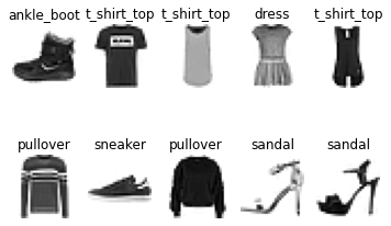
Figure 1: Fashion MNIST

Prepare Spark DataFrame for tf_images

We need to reshape our dataset so that we can store it correctly later, so we'll create two temporary Numpy Arrays, as follows:

     Python 
   
   train_images_saved = train_images.reshape((train_images.shape[0], -1))
test_images_saved = test_images.reshape((test_images.shape[0], -1))

We can check the shapes:

     Python 
   
   print("train_images_saved: " + str(train_images_saved.shape))
print("test_images_saved:  " + str(test_images_saved.shape))

The result should be:

     Python 
   
   train_images_saved: (60000, 784)
test_images_saved:  (10000, 784)

So, we have flattened the image structure.

Next, let's set the train and test values to match what we have stored in the use_id column of the img_use table:

     Python 
   
   train_code = 1
test_code = 2

Now we'll create two lists to match the structure of the tf_images table, as follows:

     Python 
   
 
 
   train_data = [
  (i,
   train_images_saved[i].astype(int).tolist(),
   int(train_labels[i]),
   train_code,
  ) for i in range(len(train_labels))
]

test_data = [
  (i,
   test_images_saved[i].astype(int).tolist(),
   int(test_labels[i]),
   test_code
  ) for i in range(len(test_labels))
] 
  

We can define our schema and create two Spark DataFrames, as follows:

     Python 
   
   from pyspark.sql.types import *

schema = StructType([
  StructField("img_idx", IntegerType(), True),
  StructField("img", ArrayType(IntegerType()), True),
  StructField("img_label", IntegerType(), True),
  StructField("img_use", IntegerType(), True)
])

train_df = spark.createDataFrame(train_data, schema)

test_df = spark.createDataFrame(test_data, schema)

We'll now concatenate the two DataFrames:

     Python 
   
   tf_images_df = train_df.union(test_df)

Let's check the structure of the DataFrame by showing several values:

     Python 
   
   tf_images_df.show(5)

The result should be similar to:

     Plain Text 
   
 
 
   +-------+--------------------+---------+-------+
|img_idx|                 img|img_label|img_use|
+-------+--------------------+---------+-------+
|      0|[0, 0, 0, 0, 0, 0...|        9|      1|
|      1|[0, 0, 0, 0, 0, 1...|        0|      1|
|      2|[0, 0, 0, 0, 0, 0...|        0|      1|
|      3|[0, 0, 0, 0, 0, 0...|        3|      1|
|      4|[0, 0, 0, 0, 0, 0...|        0|      1|
+-------+--------------------+---------+-------+
only showing top 5 rows 
  

We need to convert the values in the img column to a suitable format for SingleStore DB. We can do this using the following UDF:

     Python 
   
   import array, binascii

def vector_to_hex(vector):
  vector_bytes = bytes(array.array("I", vector))
  vector_hex = binascii.hexlify(vector_bytes)
  vector_string = str(vector_hex.decode())
  return vector_string

vector_to_hex = udf(vector_to_hex, StringType())

spark.udf.register("vector_to_hex", vector_to_hex)

We can apply this UDF as follows:

     Python 
   
   tf_images_df = tf_images_df.withColumn(
  "img_vector",
  vector_to_hex("img")
)

And, again, check the structure of the DataFrame:

     Python 
   
   tf_images_df.show(5)

The result should be similar to the following:

     Plain Text 
   
 
 
   +-------+--------------------+---------+-------+-------------------+
|img_idx|                 img|img_label|img_use|         img_vector|
+-------+--------------------+---------+-------+-------------------+
|      0|[0, 0, 0, 0, 0, 0...|        9|      1|0000000000000000...|
|      1|[0, 0, 0, 0, 0, 1...|        0|      1|0000000000000000...|
|      2|[0, 0, 0, 0, 0, 0...|        0|      1|0000000000000000...|
|      3|[0, 0, 0, 0, 0, 0...|        3|      1|0000000000000000...|
|      4|[0, 0, 0, 0, 0, 0...|        0|      1|0000000000000000...|
+-------+--------------------+---------+-------+-------------------+
only showing top 5 rows 
  

We can now drop the img column:

     Python 
   
   tf_images_df = tf_images_df.drop("img")

Create a Model

Now we are ready to process our original train and test data. First, we'll scale the values between 0 and 1, as follows:

     Python 
   
   train_images = train_images / 255.0
test_images = test_images / 255.0

Next, we'll build our model:

     Python 
   
 
 
   model = keras.Sequential(layers = [
  keras.layers.Flatten(input_shape = (28, 28)),
  keras.layers.Dense(128, activation = "relu"),
  keras.layers.Dense(10, activation = "softmax")
])

model.compile(optimizer = "adam",
              loss = "sparse_categorical_crossentropy",
              metrics = ["accuracy"]
             )

model.summary() 
  

The result should be similar to the following:

     Plain Text 
   
 
 
   Model: "sequential"
_________________________________________________________________
Layer (type)                 Output Shape              Param #    
=================================================================
flatten (Flatten)            (None, 784)               0         
_________________________________________________________________
dense (Dense)                (None, 128)               100480    
_________________________________________________________________
dense_1 (Dense)              (None, 10)                1290      
=================================================================
Total params: 101,770 Trainable params: 101,770 Non-trainable
params: 0 
  

Now we'll apply this model to the training data:

     Python 
   
 
 
   history = model.fit(train_images,
                    train_labels,
                    batch_size = 60,
                    epochs = 10,
                    validation_split = 0.2,
                    verbose = 2) 
  

The result should be similar to:

     Plain Text 
   
 
 
   Epoch 1/10
800/800 - 4s - loss: 0.5326 - accuracy: 0.8149 - val_loss: 0.4358 - val_accuracy: 0.8503
Epoch 2/10
800/800 - 3s - loss: 0.4029 - accuracy: 0.8577 - val_loss: 0.3818 - val_accuracy: 0.8627
Epoch 3/10
800/800 - 3s - loss: 0.3600 - accuracy: 0.8702 - val_loss: 0.3740 - val_accuracy: 0.8683
Epoch 4/10
800/800 - 3s - loss: 0.3325 - accuracy: 0.8782 - val_loss: 0.3863 - val_accuracy: 0.8578
Epoch 5/10
800/800 - 3s - loss: 0.3137 - accuracy: 0.8861 - val_loss: 0.3603 - val_accuracy: 0.8686
Epoch 6/10
800/800 - 3s - loss: 0.2988 - accuracy: 0.8917 - val_loss: 0.3415 - val_accuracy: 0.8748
Epoch 7/10
800/800 - 3s - loss: 0.2836 - accuracy: 0.8962 - val_loss: 0.3270 - val_accuracy: 0.8837
Epoch 8/10
800/800 - 3s - loss: 0.2719 - accuracy: 0.9010 - val_loss: 0.3669 - val_accuracy: 0.8748
Epoch 9/10
800/800 - 3s - loss: 0.2612 - accuracy: 0.9034 - val_loss: 0.3311 - val_accuracy: 0.8806
Epoch 10/10
800/800 - 3s - loss: 0.2527 - accuracy: 0.9072 - val_loss: 0.3143 - val_accuracy: 0.8892 
  

We can see the model accuracy improving over time, and we can create a plot:

     Python 
   
   plt.title("Model Accuracy")

plt.xlabel("Epoch")
plt.ylabel("Accuracy")

plt.plot(history.history["accuracy"])
plt.plot(history.history["val_accuracy"])

plt.legend(["Train", "Validation"])

plt.show()

The result should be similar to Figure 2.

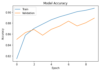
Figure 2: Model Accuracy

Alternatively, we can plot the model loss:

     Python 
   
   plt.title("Model Loss")

plt.xlabel("Epoch")
plt.ylabel("Loss")

plt.plot(history.history["loss"])
plt.plot(history.history["val_loss"])

plt.legend(["Train", "Validation"])

plt.show()

The result should be similar to Figure 3.

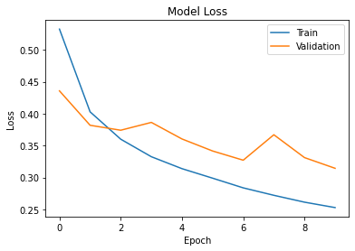
Figure 3: Model Loss

The accuracy on the test data:

     Python 
   
   (loss, accuracy) = model.evaluate(test_images, test_labels, verbose = 2)

appears good:

     Plain Text 
   
   313/313 - 1s - loss: 0.3441 - accuracy: 0.8804

Let's use the model to make predictions and look at one set of predictions:

     Python 
   
   predictions = model.predict(test_images)

print(predictions[0])

The result should be similar to:

     Plain Text 
   
   [1.4662313e-06 3.3972729e-08 2.6234572e-06 3.2284215e-06
2.3253973e-05 1.0144556e-02 4.5736870e-05 1.1021643e-01
1.2890605e-05 8.7954974e-01]

We can create a Confusion Matrix to get some more insights.

First, we’ll create categorical values:

     Python 
   
   from sklearn.metrics import confusion_matrix
from keras.utils import np_utils

cm = confusion_matrix(
  np.argmax(np_utils.to_categorical(test_labels, num_classes), axis = 1),
  np.argmax(predictions, axis = 1)
)

Next, we'll use Plotly and a solution outlined on Stack Overflow:

     Python 
   
 
 
   import plotly.graph_objects as go

data = go.Heatmap(
  z = cm[::-1],
  x = classes,
  y = classes[::-1].copy(),
  colorscale = "Reds"
)

annotations = []
thresh = cm.max() / 2

for i, row in enumerate(cm):
  for j, value in enumerate(row):
    annotations.append(
      {
        "x" : classes[j],
        "y" : classes[i],
        "font" : {"color" : "white" if value > thresh else "black"},
        "text" : str(value),
        "xref" : "x1",
        "yref" : "y1",
        "showarrow" : False
      }
    )
    
layout = {
  "title" : "Confusion Matrix",
  "xaxis" : {"title" : "Predicted"},
  "yaxis" : {"title" : "True"},
  "annotations" : annotations
}

fig = go.Figure(data = data, layout = layout)
fig.show() 
  

The result should be similar to Figure 4.

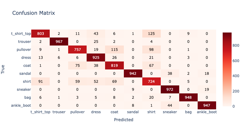
Figure 4: Confusion Matrix

We can see that the model is less accurate for some fashion items. This is because items may appear quite similar, such as Shirts and T-Shirts.

We can also plot precision and recall. First, precision:

     Python 
   
 
 
   import plotly.express as px
from sklearn.metrics import precision_score

precision_scores = precision_score(
  np.argmax(np_utils.to_categorical(test_labels, num_classes), axis = 1),
  np.argmax(predictions, axis = 1),
  average = None
)

fig = px.bar(precision_scores,
             x = classes,
             y = precision_scores,
             labels = dict(x = "Classes", y = "Precision"),
             title = "Precision Scores")

fig.update_xaxes(tickangle = 45)
fig.show() 
  

The result should be similar to Figure 5.

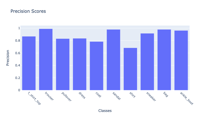
Figure 5: Precision

Now recall:

     Python 
   
 
 
   from sklearn.metrics import recall_score

recall_scores = recall_score(
  np.argmax(np_utils.to_categorical(test_labels, num_classes), axis = 1),
  np.argmax(predictions, axis = 1),
  average = None
)

fig = px.bar(recall_scores,
             x = classes,
             y = recall_scores,
             labels = dict(x = "Classes", y = "Recall"),
             title = "Recall Scores")

fig.update_xaxes(tickangle = 45)
fig.show() 
  

The result should be similar to Figure 6.

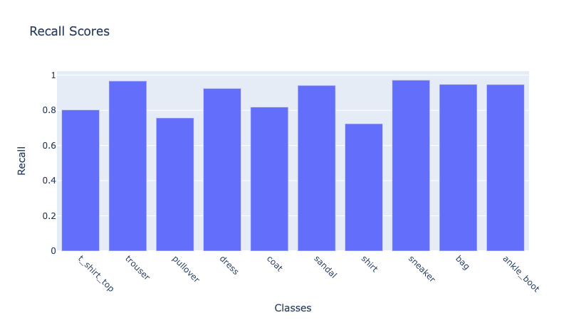
Figure 6: Recall

Prepare Spark DataFrame for prediction_results

Now we'll create a list to match the structure of the prediction_results table, as follows:

     Python 
   
 
 
   prediction_results = [
  (i,
   predictions[i].astype(float).tolist(),
   int(test_labels[i]),
   test_code
  )
  for i in range(len(test_labels))
] 
  

We can define our schema and create the Spark DataFrame, as follows:

     Python 
   
 
 
   prediction_schema = StructType([
  StructField("img_idx", IntegerType()),
  StructField("prediction_results", ArrayType(FloatType())),
  StructField("img_label", IntegerType()),
  StructField("img_use", IntegerType())
])

prediction_results_df = spark.createDataFrame(prediction_results, prediction_schema) 
  

Let's check the structure of the DataFrame by showing several values:

     Python 
   
   prediction_results_df.show(5)

The result should be similar to:

     Plain Text 
   
 
 
   +-------+--------------------+---------+-------+
|img_idx|  prediction_results|img_label|img_use|
+-------+--------------------+---------+-------+
|      0|[1.4662313E-6, 3....|        9|      2|
|      1|[2.3188923E-5, 6....|        2|      2|
|      2|[1.30073765E-8, 1...|        1|      2|
|      3|[7.774254E-7, 0.9...|        1|      2|
|      4|[0.11555459, 2.09...|        6|      2|
+-------+--------------------+---------+-------+
only showing top 5 rows 
  

We'll now create a separate column for each of the values in the prediction_results column based upon the ten fashion categories:

     Python 
   
   import pyspark.sql.functions as F

prediction_results_df = prediction_results_df.select(
  ["img_idx", "img_label", "img_use"] + [F.col("prediction_results")[i] for i in range(num_classes)]
)

col_names = ["img_idx", "img_label", "img_use"] + [classes[i] for i in range(num_classes)]

prediction_results_df = prediction_results_df.toDF(*col_names)

Write Spark DataFrames to SingleStore DB

We are now ready to write the DataFrames tf_images_df and prediction_results_df to the tables tf_images and prediction_results, respectively.

First, we'll set up the connection to SingleStore DB:

     Shell 
   
   %run ./Setup

In the Setup notebook, we need to ensure that the server address and password have been added for our SingleStore DB Cloud cluster.

In the next code cell, we'll set some parameters for the SingleStore Spark Connector, as follows:

     Python 
   
   spark.conf.set("spark.datasource.singlestore.ddlEndpoint", cluster)
spark.conf.set("spark.datasource.singlestore.user", "admin")
spark.conf.set("spark.datasource.singlestore.password", password)
spark.conf.set("spark.datasource.singlestore.disablePushdown", "false")

Finally, we are ready to write the DataFrames to SingleStore DB using the Spark Connector. First, tf_images:

     Python 
   
 
 
   (tf_images_df.write
   .format("singlestore")
   .option("loadDataCompression", "LZ4")
   .mode("ignore")
   .save("ml.tf_images")) 
  

and then prediction_results:

     Python 
   
 
 
   (prediction_results_df.write
   .format("singlestore")
   .option("loadDataCompression", "LZ4")
   .mode("ignore")
   .save("ml.prediction_results")) 
  

Example Queries

Now that we have built our system, we can run some queries. We'll include some examples from the two-part series mentioned earlier.

First, let's find how many images we have stored in tf_images:

     SQL 
   
   SELECT COUNT(*) AS count
FROM tf_images;

The result should be:

     Plain Text 
   
 
 
   +-----+
|count|
+-----+
|70000|
+-----+ 
  

Now let's take a look at some rows:

     SQL 
   
   SELECT *
FROM tf_images
LIMIT 5;

The result should be similar to:

     Plain Text 
   
 
 
   +-------+---------+-------+--------------------+
|img_idx|img_label|img_use|          img_vector|
+-------+---------+-------+--------------------+
|      0|        9|      1|00000000000000000...|
|      1|        0|      1|00000000000000000...|
|      2|        0|      1|00000000000000000...|
|      3|        3|      1|00000000000000000...|
|      4|        0|      1|00000000000000000...|
+-------+---------+-------+--------------------+ 
  

We can check the img_use table:

     SQL 
   
   SELECT use_name AS Image_Role, use_desc AS Description
FROM img_use;

The result should be:

     Plain Text 
   
 
 
   +----------+--------------------+
|Image_Role|         Description|
+----------+--------------------+
|  Training|The image is used...|
|   Testing|The image is used...|
+----------+--------------------+ 
  

The categories can be found as follows:

     SQL 
   
   SELECT class_name AS Class_Name
FROM categories;

The result should be:

     Plain Text 
   
 
 
   +-----------+
| Class_Name|
+-----------+
|t_shirt_top|
|   pullover|
|    trouser|
|    sneaker|
|     sandal|
|      shirt|
|        bag|
| ankle_boot|
|      dress|
|       coat|
+-----------+ 
  

We can also find the different fashion items:

     SQL 
   
 
 
   SELECT cn.class_name AS Class_Name,
     iu.use_name AS Image_Use,
     img_vector AS Vector_Representation
FROM tf_images AS ti
     INNER JOIN categories AS cn ON ti.img_label = cn.class_idx
     INNER JOIN img_use AS iu ON ti.img_use = iu.use_id
LIMIT 5; 
  

The result should be:

     Plain Text 
   
 
 
   +-----------+---------+---------------------+
| Class_Name|Image_Use|Vector_Representation|
+-----------+---------+---------------------+
| ankle_boot| Training| 00000000000000000...|
|t_shirt_top| Training| 00000000000000000...|
|t_shirt_top| Training| 00000000000000000...|
|      dress| Training| 00000000000000000...|
|t_shirt_top| Training| 00000000000000000...|
+-----------+---------+---------------------+ 
  

and get a summary of the number of training and testing images:

     SQL 
   
 
 
   SELECT class_name AS Image_Label,
     COUNT(CASE WHEN img_use = 1 THEN img_label END) AS Training_Images,
     COUNT(CASE WHEN img_use = 2 THEN img_label END) AS Testing_Images
FROM tf_images
     INNER JOIN categories ON class_idx = img_label
GROUP BY class_name; 
  

The result should be:

     Plain Text 
   
 
 
   +-----------+---------------+--------------+
|Image_Label|Training_Images|Testing_Images|
+-----------+---------------+--------------+
|     sandal|           6000|          1000|
|t_shirt_top|           6000|          1000|
|      shirt|           6000|          1000|
| ankle_boot|           6000|          1000|
|      dress|           6000|          1000|
|       coat|           6000|          1000|
|    trouser|           6000|          1000|
|   pullover|           6000|          1000|
|        bag|           6000|          1000|
|    sneaker|           6000|          1000|
+-----------+---------------+--------------+ 
  

Let's get some details about a specific image id:

     SQL 
   
   SELECT img_idx, img_label, use_name, use_desc
FROM tf_images
     INNER JOIN img_use ON use_id = img_use
WHERE use_name = 'Testing' AND img_idx = 0;

The result should be:

     Plain Text 
   
 
 
   +-------+---------+--------+--------------------+
|img_idx|img_label|use_name|            use_desc|
+-------+---------+--------+--------------------+
|      0|        9| Testing|The image is used...|
+-------+---------+--------+--------------------+ 
  

Bonus: Streamlit Visualization

We can use Streamlit to create a small application to select an image and show the model predictions.

Install the Required Software

We need to install the following packages:

     Plain Text 
   
 
 
   streamlit
matplotlib
plotly
numpy
pandas
pymysql 
  

These can be found in the requirements.txt file on GitHub. Run the file as follows:

     Shell 
   
   pip install -r requirements.txt

Example Application

Here is the complete code listing for streamlit_app.py:

     Python 
   
 
 
   # streamlit_app.py

import streamlit as st
import array
import binascii
import matplotlib.pyplot as plt
import plotly.express as px
import numpy as np
import pandas as pd
import pymysql

# Initialize connection.

def init_connection():
    return pymysql.connect(**st.secrets["singlestore"])

conn = init_connection()

def hex_to_vector(vector):
    vector_unhex = binascii.unhexlify(vector)
    vector_list = list(array.array("I", vector_unhex))
    return vector_list

img_idx = st.slider("Image Index", 0, 9999, 0)

img_df = pd.read_sql("""
SELECT img_vector
FROM tf_images
     INNER JOIN img_use ON use_id = img_use
WHERE use_name = 'Testing' AND img_idx = %s;
""", conn, params = ([str(img_idx)]))

vector_string = img_df["img_vector"][0]

img = np.array(hex_to_vector(vector_string)).reshape(28, 28)

fig = plt.figure(figsize = (1, 1))
plt.imshow(img, cmap = plt.cm.binary)
plt.axis("off")
st.pyplot(fig)

predictions_df = pd.read_sql("""
SELECT t_shirt_top, trouser, pullover, dress, coat, sandal, shirt, sneaker, bag, ankle_boot, class_name
FROM prediction_results
     INNER JOIN categories ON img_label = class_idx
WHERE img_idx = %s;
""", conn, params = ([str(img_idx)]))

classes = [
  "t_shirt_top",
  "trouser",
  "pullover",
  "dress",
  "coat",
  "sandal",
  "shirt",
  "sneaker",
  "bag",
  "ankle_boot"
]

num_classes = len(classes)

max_val = predictions_df[classes].max(axis = 1)[0]

predicted = (predictions_df[classes] == max_val).idxmax(axis = 1)[0]
actual = predictions_df["class_name"][0]

st.write("Predicted: ", predicted)
st.write("Actual: ", actual)

if (predicted == actual):
   st.write("Prediction Correct")
else:
   st.write("Prediction Incorrect")

probabilities = [predictions_df[class_name][0] for class_name in classes]

bar = px.bar(probabilities,
             x = classes,
             y = probabilities,
             color = probabilities,
             labels = dict(x = "Classes", y = "Probability"),
             title = "Prediction")

bar.update_xaxes(tickangle = 45)
bar.layout.coloraxis.colorbar.title = "Probability"

st.plotly_chart(bar)
st.table(predictions_df) 
  

Create a Secrets File

Our local Streamlit application will read secrets from a file .streamlit/secrets.toml in our application's root directory. We need to create this file as follows:

     Plain Text 
   
 
 
   # .streamlit/secrets.toml

[singlestore]
host = "<TO DO>"
port = 3306
database = "ml"
user = "admin"
password = "<TO DO>" 
  

The <TO DO> for host and password should be replaced with the values obtained from SingleStore Cloud when creating a cluster.

Run the Code

We can run the Streamlit application as follows:

     Shell 
   
   streamlit run streamlit_app.py

The output in a web browser should look like Figures 7 and 8. We can select an image by moving the slider. This will show us the predictions for that image.

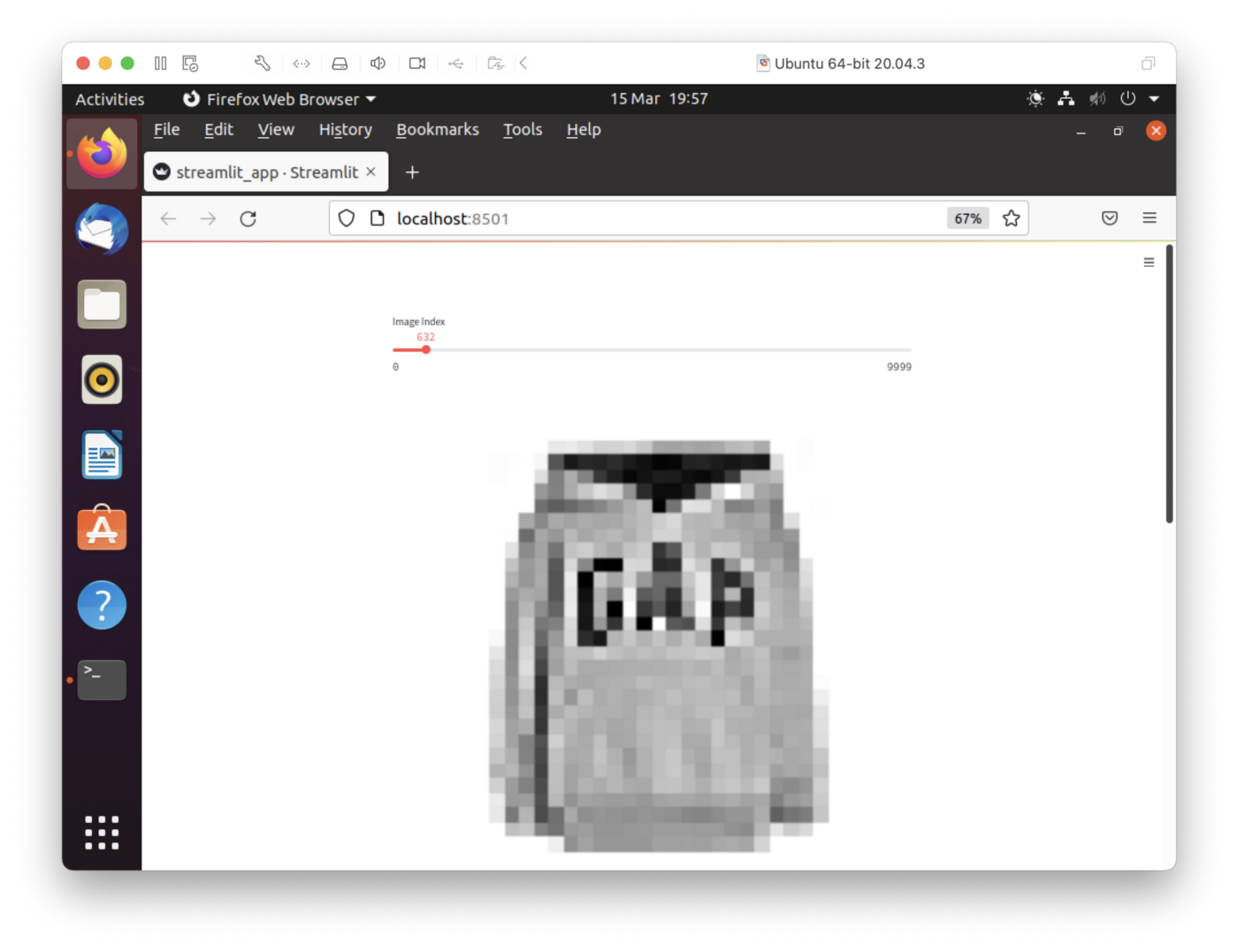
Figure 7: Streamlit (Top Half)

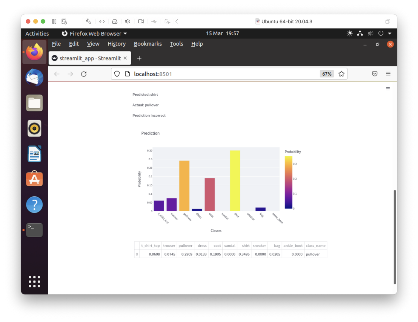
Figure 8: Streamlit (Bottom Half)

In Figure 7, we have the slider to select the image id and, in the example here, image 632 was selected. In Figure 8, we can see that the fashion item was predicted as a Shirt but was a Pullover.

Feel free to experiment with the code to suit your needs. A suggestion would be to improve the rendering of the greyscale image as it currently appears too large, as we can see in Figure 7.

Summary

In this article, we have seen how SingleStore DB can work very effectively with Keras and Tensorflow. Inside SingleStore DB, we have been able to store the test and train data as well as the model predictions. Our Streamlit application also allows us to view the predictions for an image.

Database Keras TensorFlow application Label sql Machine learning SingleStore

Published at DZone with permission of Akmal Chaudhri. See the original article here.

Opinions expressed by DZone contributors are their own.

Comments

Image Classification Using SingleStore DB, Keras, and Tensorflow

Follow along in this tutorial to learn how to store Fashion MNIST images and ML predictions in SingleStore DB.

Abstract

Introduction

Configure Databricks CE

Create Database Tables

Fill Out the Notebook

Load the Dataset

Prepare Spark DataFrame for tf_images

Create a Model

Prepare Spark DataFrame for prediction_results

Write Spark DataFrames to SingleStore DB

Example Queries

Bonus: Streamlit Visualization

Install the Required Software

Example Application

Create a Secrets File

Run the Code

Summary

Popular on DZone

Database Partner Resources