Feature Engineering Techniques That Actually Improve Model Accuracy

Most gains in a supervised learning project don't come from switching algorithms; they come from what you feed the algorithm. Feature engineering is the process of transforming raw data into representations that make patterns easier for a model to learn. Done well, it routinely closes more of the accuracy gap than hyperparameter tuning or trying a fancier model.

This article walks through the feature engineering techniques that consistently move the needle in real projects, with working Python code (pandas + scikit-learn) and a visual look at where the gains actually come from.

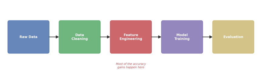
Figure 1: Where feature engineering sits in a typical supervised ML pipeline.

Why Feature Engineering Beats Model Selection (Often)

A gradient-boosted tree with well-engineered features will usually outperform a deep neural network fed raw, unprocessed columns. That's because feature engineering directly encodes domain knowledge and statistical structure that the model would otherwise have to infer from data alone — often with far more examples than you have available.

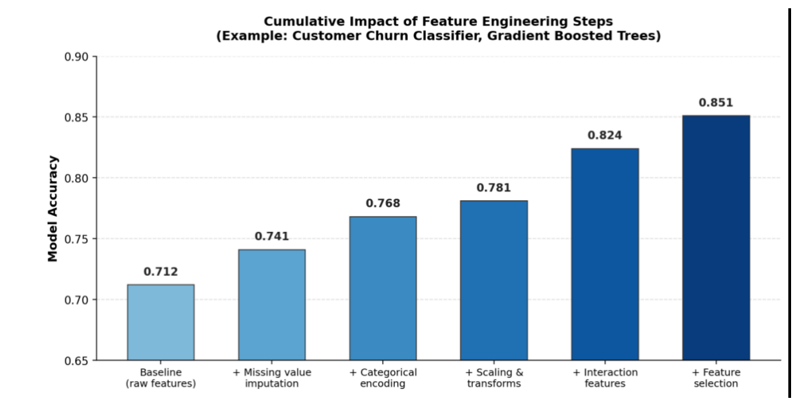
Figure 2: Cumulative accuracy gains on a churn-prediction task as each feature engineering step is added.

In this example (a customer churn classifier trained with gradient-boosted trees), accuracy climbs from 0.712 on raw features to 0.851 after five feature engineering passes, a 13.9-point improvement without changing the model or its hyperparameters.

Techniques That Actually Move the Needle

1. Missing Value Imputation (With an Indicator Flag)

Dropping rows with missing values throws away signal. Simple mean/median imputation is a safe default but pairing it with a binary "was this missing" flag preserves the fact that the value was absent, which is often itself predictive (e.g., a missing income field can correlate with churn).

import pandas as pd
from sklearn.impute import SimpleImputer
 
# Flag missingness before imputing — the flag is a feature in its own right
df['income_missing'] = df['income'].isna().astype(int)
 
imputer = SimpleImputer(strategy='median')
df['income'] = imputer.fit_transform(df[['income']])

2. Categorical Encoding (Target/Frequency, Not Just One-Hot)

One-hot encoding works fine for low-cardinality columns, but it explodes dimensionality for high-cardinality categoricals (zip codes, product IDs). Target encoding, replacing a category with the mean target value for that category, keeps dimensionality flat and often outperforms one-hot for tree-based models. Always fit encodings on the training fold only to avoid leakage.

from category_encoders import TargetEncoder
from sklearn.model_selection import KFold
 
encoder = TargetEncoder(cols=['zip_code'], smoothing=0.3)
 
# Fit only on training data, then apply to validation/test
encoder.fit(X_train['zip_code'], y_train)
X_train['zip_code_enc'] = encoder.transform(X_train['zip_code'])
X_valid['zip_code_enc'] = encoder.transform(X_valid['zip_code'])

3. Scaling and Skew Correction

Distance-based and linear models (KNN, SVM, logistic regression) are sensitive to feature scale; tree-based models are not, but still benefit from skew correction. A log transform on heavily right-skewed features (income, transaction amounts) tightens the distribution and reduces the influence of outliers.

import numpy as np
from sklearn.preprocessing import StandardScaler
 
# Log-transform skewed monetary features (add 1 to handle zeros)
df['txn_amount_log'] = np.log1p(df['txn_amount'])
scaler = StandardScaler()
num_cols = ['age', 'tenure_months', 'txn_amount_log']
df[num_cols] = scaler.fit_transform(df[num_cols])

4. Interaction and Ratio Features

Models capture linear or split-based patterns per feature; they don't automatically discover that the ratio of two columns is what matters. Manually creating interaction terms and ratios spend-per-visit, tenure-to-age ratio gives the model shortcuts to patterns it would otherwise need many more splits or much more data to approximate.

# Ratio feature: average spend per visit is often more predictive
# than either 'total_spend' or 'visit_count' alone
df['spend_per_visit'] = df['total_spend'] / df['visit_count'].replace(0, 1)
 
# Interaction: tenure relative to customer age
df['tenure_ratio'] = df['tenure_months'] / (df['age'] * 12)

5. Date/Time Decomposition

A raw timestamp is nearly useless to a model. Decomposing it into cyclical and calendar components day of week, month, is-weekend, sine/cosine encodings for cyclical features exposes seasonality and recurring patterns that the model can actually split on.

df['signup_date'] = pd.to_datetime(df['signup_date'])
df['signup_dow'] = df['signup_date'].dt.dayofweek
df['signup_month'] = df['signup_date'].dt.month
df['is_weekend'] = (df['signup_dow'] >= 5).astype(int)
 
# Cyclical encoding so December and January are 'close' to the model
df['month_sin'] = np.sin(2 * np.pi * df['signup_month'] / 12)
df['month_cos'] = np.cos(2 * np.pi * df['signup_month'] / 12)

6. Feature Selection (Prune After You Expand)

Adding interaction and encoded features inflates dimensionality, which can reintroduce noise and overfitting. Closing the loop with feature selection, dropping low-importance or highly correlated features, is what typically delivers the last, and sometimes largest, accuracy gain in the pipeline.

from sklearn.feature_selection import SelectFromModel
from sklearn.ensemble import GradientBoostingClassifier
 
base_model = GradientBoostingClassifier(random_state=42)
base_model.fit(X_train, y_train)
 
# Keep only features with above-median importance
selector = SelectFromModel(base_model, threshold='median', prefit=True)
X_train_selected = selector.transform(X_train)
X_valid_selected = selector.transform(X_valid)
 
print(f'Kept {X_train_selected.shape[1]} of {X_train.shape[1]} features')

Common pitfall: fitting imputers, encoders, and scalers on the full dataset before splitting into train/test. This leaks information from the validation set into training and inflates your reported accuracy. Always fit transformations on the training fold only, inside a cross-validation loop or an sklearn Pipeline.

Putting It Together: Before vs. After

The table below summarizes the cumulative effect of each technique from the churn-prediction example, holding the model (gradient boosted trees, default hyperparameters) constant throughout.

Wrapping It in a Reproducible Pipeline

Scattered feature engineering code is a common source of train/serve skew. Wrapping the steps in an sklearn Pipeline (or ColumnTransformer) keeps fitting and transforming consistent between training and inference, and makes the whole thing a single object you can version and deploy.

from sklearn.pipeline import Pipeline
from sklearn.compose import ColumnTransformer
from sklearn.impute import SimpleImputer
from sklearn.preprocessing import StandardScaler
from category_encoders import TargetEncoder
from sklearn.ensemble import GradientBoostingClassifier
 
numeric_features = ['age', 'tenure_months', 'txn_amount_log']
categorical_features = ['zip_code']
 
preprocessor = ColumnTransformer(transformers=[
    ('num', Pipeline([
        ('impute', SimpleImputer(strategy='median')),
        ('scale', StandardScaler()),
    ]), numeric_features),
    ('cat', TargetEncoder(), categorical_features),
])
 
full_pipeline = Pipeline([('preprocess', preprocessor),
    ('model', GradientBoostingClassifier(random_state=42)),
])
 
full_pipeline.fit(X_train, y_train)
print(full_pipeline.score(X_valid, y_valid))

Best Practices Checklist

• Always fit transformers (imputers, encoders, scalers) on the training fold only, never on the full dataset before splitting.
• Flag missingness explicitly instead of silently imputing; the flag itself often carries signal.
•  Prefer target/frequency encoding over one-hot for high-cardinality categorical columns.
•  Log-transform heavily skewed numeric features before scaling.
•  Create interaction and ratio features that reflect domain knowledge, not random combinations.
•  Decompose timestamps into calendar and cyclical components rather than using raw dates.
•  Re-run feature selection after adding new engineered features to control dimensionality and overfitting.
•  Wrap the whole process in a pipeline/column transformer so training and inference stay in sync.

Conclusion

Feature engineering is unglamorous compared to trying the newest architecture, but it's usually the highest-leverage work in a supervised learning project. Handle missing data deliberately, encode categoricals to fit their cardinality, correct skew, build interactions that reflect real relationships in your domain, decompose dates, and prune what you don't need. In the example walked through here, that sequence alone was responsible for nearly 14 points of accuracy, with the model and hyperparameters held constant the entire time.