Implementing ΔE-ITP in Python: Accurate Color Difference Metric for Image Processing

Image difference analysis is essential in computer vision, graphics processing, and media quality assessment. Whether you're evaluating compression artifacts, detecting subtle regressions, or comparing perceptual similarity, various metrics help quantify differences between images.

This article discusses popular image difference metrics, their pros and cons, and recommends ΔE-ITP, a modern, perceptually optimized color difference metric. We’ll also look at how to implement DeltaE ITP—including transforming images from SDR, HLG, and PQ into ITP—and interpreting the reported color differences effectively.

Popular Image Difference Metrics

1. Mean Squared Error (MSE)

MSE calculates the average of the squared differences between corresponding pixels:

MSE = (1/N) * Σ (I1 - I2)^2

Pros:

• Simple to compute
• Useful for detecting basic structural differences

Cons:

• Ignores human visual perception
• Sensitive to small brightness or noise variations

2. Peak Signal-to-Noise Ratio (PSNR)

Derived from MSE, PSNR measures the ratio of signal strength to noise in decibels:

PSNR = 10 * log10(MAX^2 / MSE)

Interpretation (approximate percentage match):

• > 30 dB ≈ 90–100% match (imperceptible differences)
• 20–30 dB ≈ 60–90% match (visible differences)
• < 20 dB ≈ <60% match (noticeable distortion)

Pros:

• Commonly used in compression benchmarking
• Simple and interpretable

Cons:

• Weak correlation with perceptual quality
• Ignores chromaticity and structural variation

3. Structural Similarity Index (SSIM)

SSIM improves on MSE/PSNR by comparing luminance, contrast, and structure:

SSIM(x, y) = [(2μxμy + C1)(2σxy + C2)] / [(μx² + μy² + C1)(σx² + σy² + C2)]

Pros:

• Better aligns with human visual perception
• Evaluates structural and luminance consistency

Cons:

• Sensitive to image scale and contrast
• Less effective for color differences

CIE Color Model: The Foundation of Perceptual Metrics

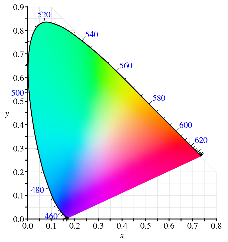
To understand perceptual color difference, we must start with the CIE color model. Developed in 1931 by the International Commission on Illumination (CIE), it standardizes color based on human vision. Derived from psychophysical experiments, the CIE 1931 XYZ color space represents color as combinations of three stimuli (X, Y, Z).

• X ≈ red perception
• Y ≈ brightness (luminance)
• Z ≈ blue perception

Later extensions like CIE Lab (1976) and CIE Luv introduced perceptual uniformity, critical for color difference calculations like ΔE.

4. ΔE-2000

This metric quantifies perceptual color differences in CIELAB space, improving on earlier ΔE formulas by adjusting for hue, chroma, and lightness.

Pros:

• Better matches human perception
• Widely used in print, manufacturing, and SDR content
• Compatible with legacy color workflows

Cons:

• Inaccurate for HDR or wide color gamut (WCG)
• Struggles with extreme saturation or very low luminance (with nits values around 0.1 cd/m2 )

5. ΔE-ITP: A Modern Color Difference Metric

Introduced in 2019 via ITU-R BT.2124, DeltaE ITP was built for HDR and WCG—where ΔE-2000 falls short. It's based on the ICtCp color space from Rec. 2100, offering greater perceptual uniformity across brightness and saturation extremes.

Why ΔE-ITP?

• ΔE-2000 fails under low (<1 cd/m²) or high (>100 cd/m²) luminance
• Underestimates differences in certain hues (e.g., BT.709 blue)

How It's Computed:

1. Convert from Rec. 709, HLG, or PQ → Rec. 2020 Display Linear
2. Convert to LMS (Long, Medium, Short cone responses)
3. Map LMS → ICtCp
4. Compute Euclidean distance in ITP space

Color Space Explanations

LMS Color Space

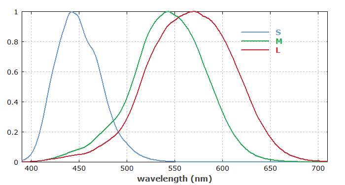
• L: Long wavelengths (reds)
• M: Medium (greens)
• S: Short (blues/violets)

ICtCp (ITP)

ICTCP is a modern color space developed for high dynamic range (HDR) and wide color gamut (WCG) video, standardized in ITU-R Rec. 2100. It improves upon traditional color spaces like YCbCr by offering better perceptual uniformity, reduced hue distortion, and more efficient chroma subsampling—key benefits for HDR content. 

ICTCP consists of three components: 

I (Intensity) - representing perceptual brightness based on human vision;

CT - capturing the red-green chromatic difference;

CP - capturing the blue-yellow chromatic difference. 

These components are derived from Rec. 2020 RGB using HDR perceptual transfer functions (PQ or HLG) and LMS cone response modeling, enabling more accurate and efficient color representation for modern displays.

Comparing ΔE-2000 vs. ΔE-ITP

Why ΔE-ITP Is Superior

• Accurate under extreme luminance and saturation
• Works across SDR, HDR, and WCG
• Closely follows human perception in modern display environments

Writing Your Own ΔE-ITP Image Difference Metric

Step 1: Read Images and Convert to Display Linear RGB

To accurately process images for perceptual difference metrics, it's essential to identify their color space and transfer function. Most standard images (e.g., PNG, JPEG) use sRGB/Rec.709 with a gamma curve, while HDR images may use Rec.2020 with PQ (ST.2084) or HLG. After identifying the colorspace of the input media apply the correct inverse transfer function to convert the image to Rec.2020 display-linear RGB, ensuring accurate color interpretation for further analysis. 

Below are code blocks for converting from the mentioned colorspaces to display linear RGB.

Converting Rec 709 Gamma to Rec 2020 Display Nits

import numpy as np

def rec709_to_rec2020_display_nits(rgb709):
    """
    Convert Rec.709 gamma-encoded RGB to Rec.2020 display-linear RGB in nits.

    Args:
        rgb709 (array): Gamma-encoded Rec.709 RGB values (range 0–1).

    Returns:
        Output: Rec.2020 display-linear RGB values scaled to 100 nits.
    """
    rgb709 = np.asarray(rgb709)

    # Step 1: Gamma decode (Rec.709 OETF ~ gamma 2.4)
    gamma = 2.4
    rgb_linear_709 = np.power(rgb709, gamma)

    # Step 2: Convert from Rec.709 linear to Rec.2020 linear
    # Matrix from Rec.709 to Rec.2020 (approximate, normalized RGB conversion)
    M_709_to_2020 = np.array([
        [1.6605, -0.5876, -0.0728],
        [-0.1246, 1.1329, -0.0083],
        [-0.0182, -0.1006, 1.1187]
    ])

    rgb_linear_2020 = M_709_to_2020 @ rgb_linear_709

    # Step 3: Scale so that 1.0 linear = 100 nits
    rgb_nits = rgb_linear_2020 * 100.0

    return rgb_nits

 Converting PQ to Rec 2020 Display Nits

import numpy as np
from colour.models import eotf_inverse_ST2084

def pq_to_display_linear_rgb2020(rgb_pq, peak_luminance=10000.0):
    """
    Convert PQ-encoded RGB to Rec.2020 display-linear RGB (normalized 0–1).

    Args:
        rgb_pq (array): PQ-encoded RGB values (range 0–1).
        peak_luminance (float): Maximum display luminance in nits (default: 10000 nits for PQ).

    Returns:
        Output: Display-linear RGB values normalized to 0–1.
    """
    rgb_pq = np.asarray(rgb_pq)

    # Decode PQ to absolute luminance in nits
    rgb_nits = eotf_inverse_ST2084(rgb_pq)

    # Normalize to [0, 1] by dividing by peak luminance
    rgb_display_linear = rgb_nits / peak_luminance

    return rgb_display_linear

Converting HLG to Rec 2020 Display Nits

import numpy as np
from colour.models import eotf_inverse_ARIBSTDB67

def hlg_to_display_nits(rgb_hlg, peak_luminance=1000.0):
    """
    Convert HLG-encoded RGB to Rec.2020 display-linear RGB in nits.

    Args:
        rgb_hlg (array-like): HLG-encoded RGB values (range 0–1).
        peak_luminance (float): Peak luminance of the display (default 1000 nits).

    Returns:
        Output: Display-linear RGB values in nits.
    """
    rgb_hlg = np.asarray(rgb_hlg)

    # Decode HLG to relative linear light (0–1)
    rgb_linear = eotf_inverse_ARIBSTDB67(rgb_hlg)

    # Scale to absolute luminance in nits
    rgb_nits = rgb_linear * peak_luminance

    return rgb_nits

Step 2: Convert Display Linear Nits to LMS

def rgb_to_lms(rgb):
    """
    Convert Rec.2020 display linear RGB to LMS (cone response domain).
    
    Args:
        rgb (array-like): 3-element array of linear RGB values [R, G, B], range [0, 1]

    Returns:
        np.ndarray: 3-element array [L, M, S]
    """
    rgb = np.asarray(rgb)

    # RGB to LMS matrix from ITU-R BT.2100
    M_RGB_to_LMS = np.array([
        [ 0.3592,  0.6976, -0.0358],
        [-0.1922,  1.1004,  0.0755],
        [ 0.0069,  0.0749,  0.8434]
    ])

    # Multiply RGB vector by the matrix
    lms = M_RGB_to_LMS @ rgb

    return lms

Step 3: Convert LMS to L'M'S' With PQ Non Linearity defined With ST-2084

import numpy as np
from colour.models import eotf_ST2084

def lms_to_inverse_lms_pq(lms, peak_luminance=10000):
    """
    Convert LMS (display-linear in nits) to inverse LMS using PQ non-linearity.

    Args:
        lms (array): LMS values in display-linear light (nits).
        peak_luminance (float): PQ peak luminance, usually 10000 nits.

    Returns:
         Inverse LMS.
    """
    lms = np.asarray(lms)

    # Normalize LMS to 0–1 based on peak luminance
    lms_normalized = lms / peak_luminance

    # Apply ST2084 EOTF
    lms_inverse = eotf_ST2084(lms_normalized)

    return lms_inverse

Step 4: Convert Inverse LMS to ITP

import numpy as np

def inverse_lms_to_itp(inverse_lms):
    """
    Convert inverse LMS (PQ-encoded) to ICtCp (ITP space).

    Args:
        inverse_lms (array-like): 3-element PQ-encoded inverse LMS values [L, M, S]

    Returns:
        np.ndarray: 3-element ICtCp values [I, Ct, Cp]
    """
    inverse_lms = np.asarray(inverse_lms)

    # Matrix: LMS → ICtCp (from ITU-R BT.2100)
    M_LMS_to_ICtCp = np.array([
        [ 0.5,     0.5,     0.0    ],
        [ 1.6137, -3.3234,  1.7097 ],
        [ 4.3781, -4.2455, -0.1326 ]
    ])

    # Transform
    ictcp = M_LMS_to_ICtCp @ inverse_lms
    return ictcp

Step 5: Calculate ΔE-ITP : Distance Between Two ITP Color Values

import math

def delta_itp(color1, color2):
    """
    Calculate the ΔITP (perceptual distance) between two ICTCP values.

    Parameters:
        color1 (tuple): (I1, T1, P1) values
        color2 (tuple): (I2, T2, P2) values

    Returns:
        float: ΔITP distance
    """
    I1, T1, P1 = color1
    I2, T2, P2 = color2

    delta_I = I1 - I2
    delta_T = T1 - T2
    delta_P = P1 - P2

    return math.sqrt(delta_I**2 + delta_T**2 + delta_P**2)

# Example usage
color1 = (0.5, 0.1, -0.05)
color2 = (0.6, 0.12, -0.02)

distance = delta_itp(color1, color2)
print(f"ΔITP distance: {distance:.6f}")

Step 6: Scale the Output Score

The ΔE ITP distance is calculated as the Euclidean distance in ICtCp space, then scaled by 240 to approximate the ΔE 2000 range, or by 720 to align with just-noticeable difference (JND) units.

Image Difference Grading Thresholds

Thresholds turn raw difference scores into meaningful insights relevant to human perception:

Conclusion

Traditional metrics like MSE, PSNR, and SSIM provide basic insight into image differences but fail to capture perceptual accuracy—especially for modern HDR and wide-gamut media. DeltaE ITP, built on cutting-edge color science and the ICtCp color space, offers a more reliable, perceptually aligned approach.

By embracing ITP-based analysis and integrating visual thresholds, engineers and creatives alike can make smarter quality decisions grounded in how humans actually see.