Jeffrey Microscope for Generating Flame Graphs in Java

Java Flight Recorder (JFR) captures an enormous amount of detail about what your application is doing — but raw JFR files are only as useful as the tools you have to explore them. Jeffrey is an open-source JFR analyzer that specializes in turning JFR events into interactive visualizations, and Jeffrey Microscope is its standalone, single-user deployment: a self-contained application that lets you import recordings and dig into flamegraphs, timeseries, and other views right in your browser. Getting started takes a minute:

• Standalone JAR – download the latest microscope.jar from the GitHub releases page and start it with java -jar microscope.jar (Java 25 or newer).
• Docker – skip the setup entirely with docker run -it --network host petrbouda/microscope.
• Sample recordings – if you want to explore the tool before profiling your own application, the petrbouda/microscope-examples image ships with sample recordings preloaded (docker run -it --network host petrbouda/microscope-examples).

In this article, we'll use Jeffrey Microscope to analyze JFR flamegraphs and walk through how they help you find where your application actually spends its time.

Let's set up a hands-on environment. Download the latest microscope.jar from the GitHub releases page and launch it (Java 25 or newer):

java -jar microscope.jar

Open it in your browser, then grab some recordings to analyze — Jeffrey maintains a companion repository of real JFR recordings captured from various serialization and profiling scenarios:

git clone https://github.com/petrbouda/jeffrey-recordings

The files ship as compressed .jfr.lz4, which Jeffrey Microscope reads natively. Drag one onto the Drop Recordings zone on the dashboard — the upload starts automatically, and within a few seconds you have a profile ready to explore.

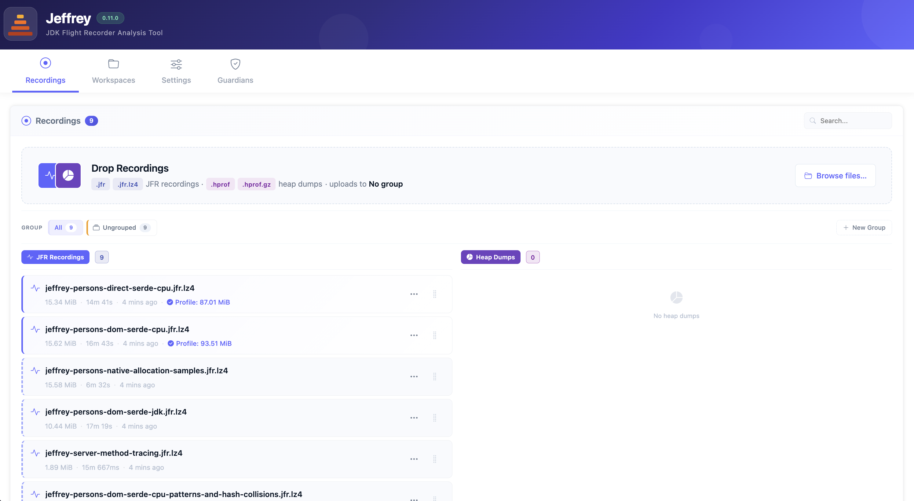
For this walkthrough, we'll focus on two recordings that profile the same piece of code — an HTTP endpoint that serializes and deserializes JSON — with one deliberate difference between them:

• jeffrey-persons-direct-serde-cpu.jfr.lz4 – the optimized path. JSON is serialized directly to and from Java objects, with additional caching in place.
• jeffrey-persons-dom-serde-cpu.jfr.lz4 – the unoptimized path. JSON is routed through a DOM representation (JsonNode) before being converted to Java objects, intentionally creating extra garbage along the way.

Because both recordings exercise the same endpoint under the same workload, they make an ideal before-and-after pair for generating flamegraphs and differential graphs, as we show later.

Exploring the Primary Flamegraphs

Let's start with the optimized recording. Click jeffrey-persons-direct-serde-cpu.jfr.lz4 to open its profile, then head to the Visualization tab and select Primary under Flamegraphs in the sidebar. Jeffrey inspects the recording and presents a card for every flamegraphable event type it found — each ready to render on its own:

• Execution Samples (jdk.ExecutionSample) – CPU profiling via perf_events, the most relevant card for a CPU profile like this one.
• Wall-Clock Samples (profiler.WallClockSample) – wall-clock time, including waiting.
• Allocation Samples (jdk.ObjectAllocationInNewTLAB) – memory allocation, weighted by object count or total bytes.
• Java Monitor Blocked, Java Thread Park, Java Monitor Wait – lock-contention and thread-parking events.

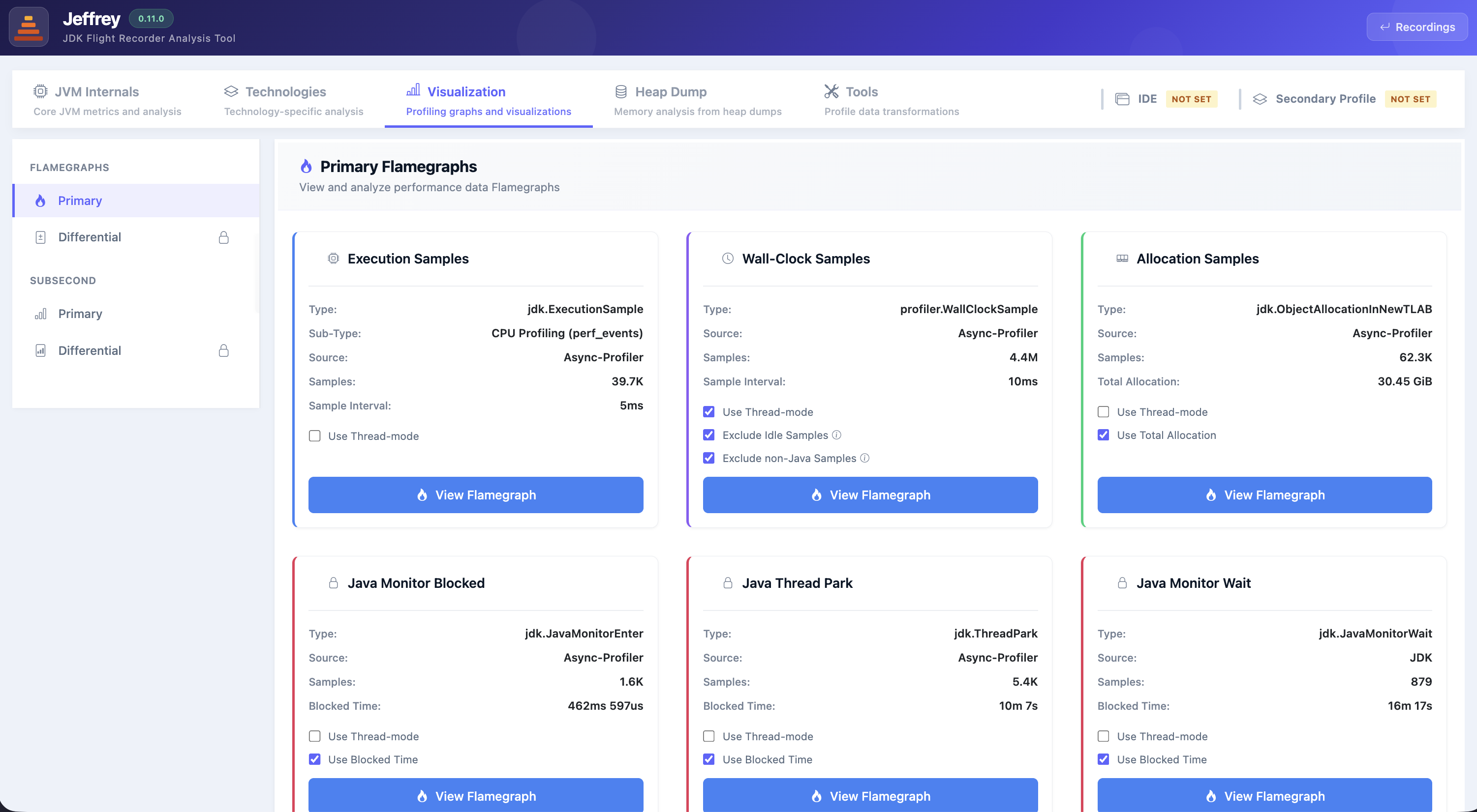
Each card shows the event type, its source (Async-Profiler or the JDK), the sample count, and a few rendering options — for example, Use Thread-mode to split the graph by thread, or Use Total Allocation to weight the allocation flamegraph by bytes rather than sample count. Click View Flamegraph on the Execution Samples card to see where the CPU time goes.

Timeseries

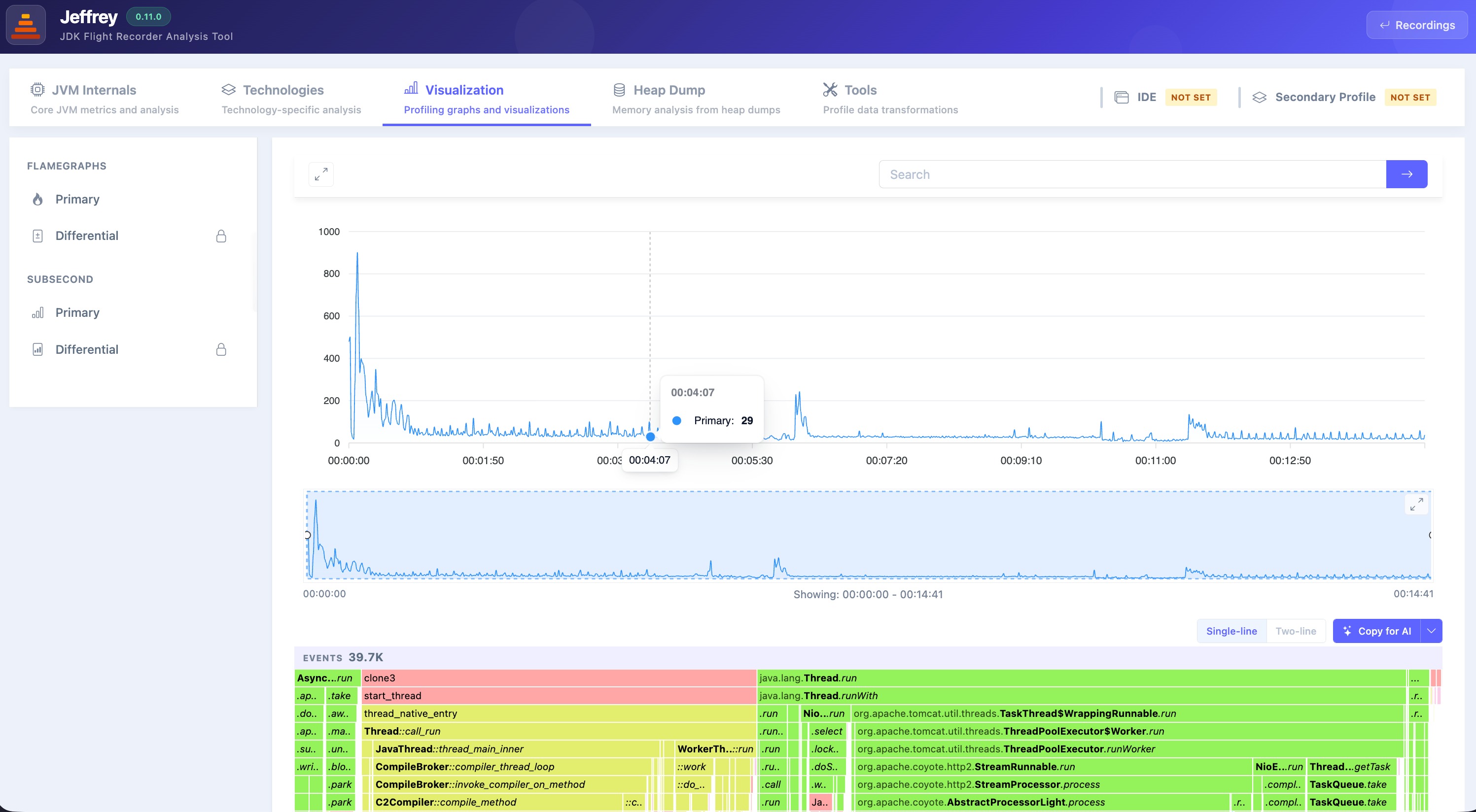
Above the flamegraph, Jeffrey plots the selected event across the recording's timeline, so you can see how activity changes over the run — warm-up, steady state, and spikes all stand out. Drag the handles on the range selector below to narrow the window, and the flamegraph rebuilds from only the samples in that interval.

Flamegraph

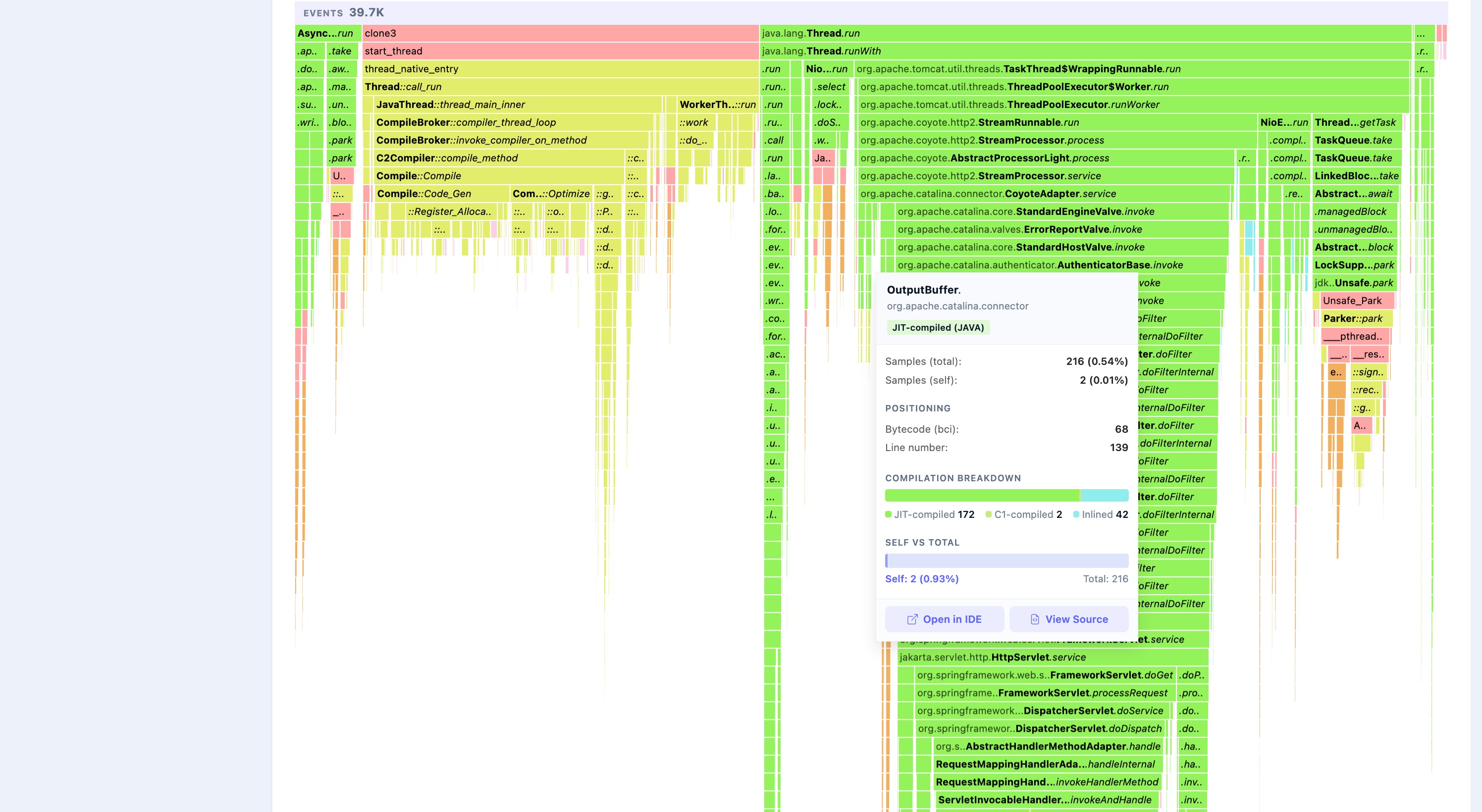
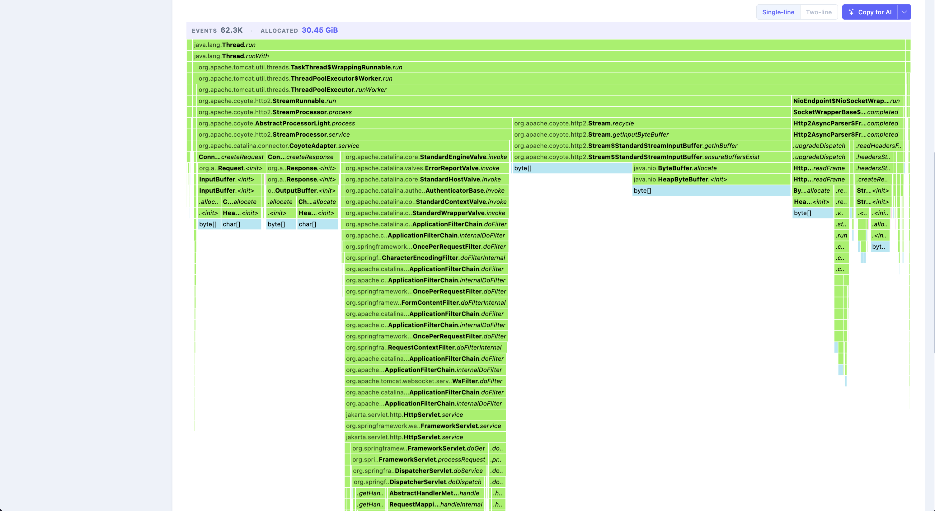
Each box is a stack frame, its width proportional to the samples that captured it, stacking upward toward the methods running on-CPU. Wide boxes are where time goes. Read top to bottom to follow the full call path from entry point down into your own code. Click any frame to zoom into that subtree.

Search

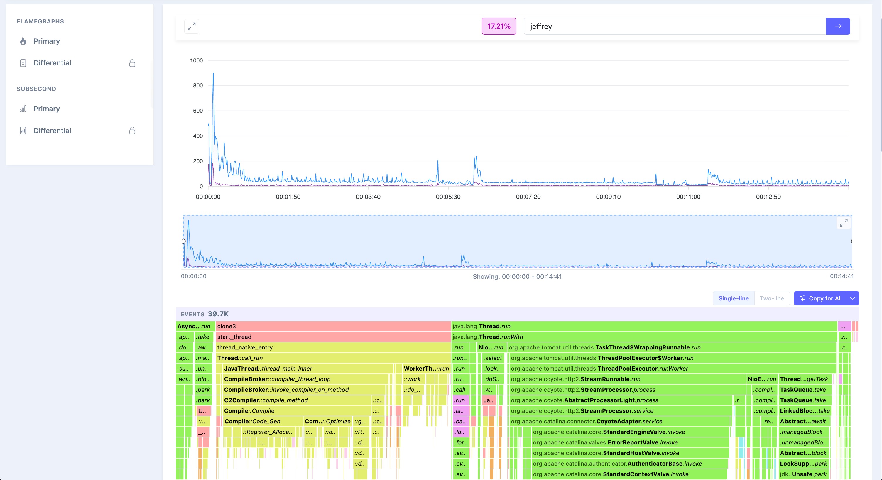
The search box highlights every frame matching your query and reports what share of the profile those matches account for — a fast way to answer "how much time is really in my code?" and to locate a method however deep it sits.

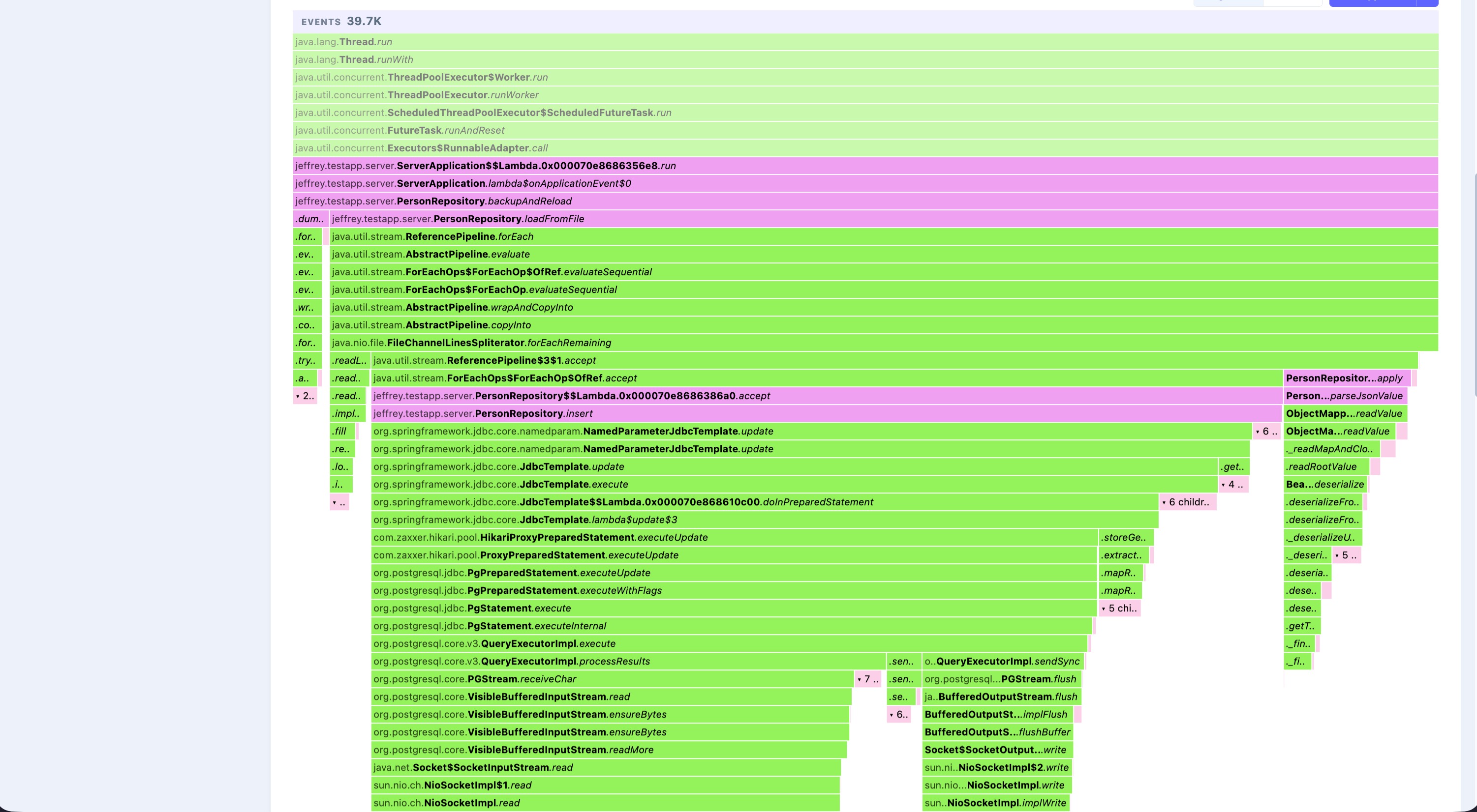
The Frame Tooltip

Hovering a frame shows far more than a sample count: total vs self samples (time through the frame vs directly in it), its bytecode index and source line, and a compilation breakdown — JIT-compiled, C1-compiled, or inlined — revealing how the method was actually executed. Open in IDE, and View Source jump straight to the code, once Microscope is paired with the Jeffrey IntelliJ plugin.

Copy for AI

The Copy for AI button exports the current view — stacks, weights, and hot paths — as a compact Markdown summary, copied to your clipboard or downloaded as .md. Paste it into e.g. Claude Code and let the AI optimize your code based on runtime profiles from flamegraphs.

Other Flamegraphs

Everything above applies to more than just CPU. Back on the Primary page, you can open the Allocation and Wall-Clock flamegraphs the same way — same navigation, search, tooltip, and range selector — but each answers a different question:

• Wall-Clock – where wall-clock time is spent, including waiting, rather than just on-CPU work.
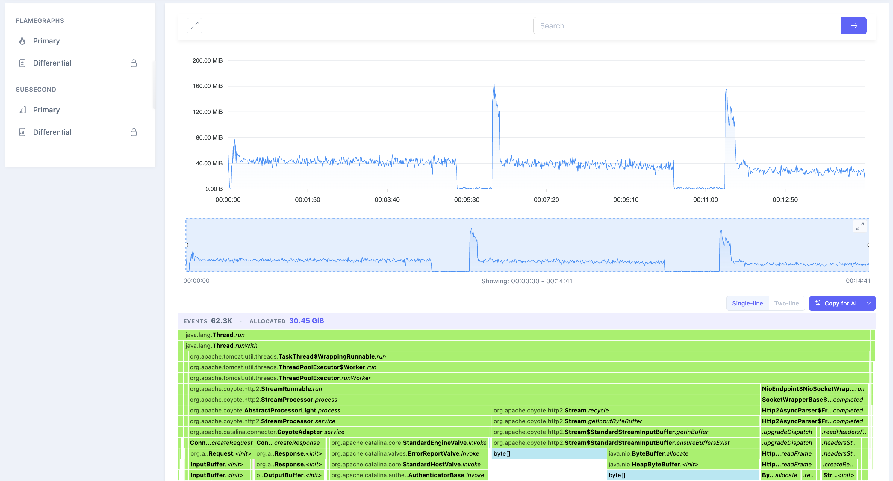
• Allocation – where memory is allocated.

Two rendering options are worth trying:

• Use Thread-mode – splits the graph by thread, showing per-thread call trees instead of one merged view. Handy when a single thread dominates or misbehaves.

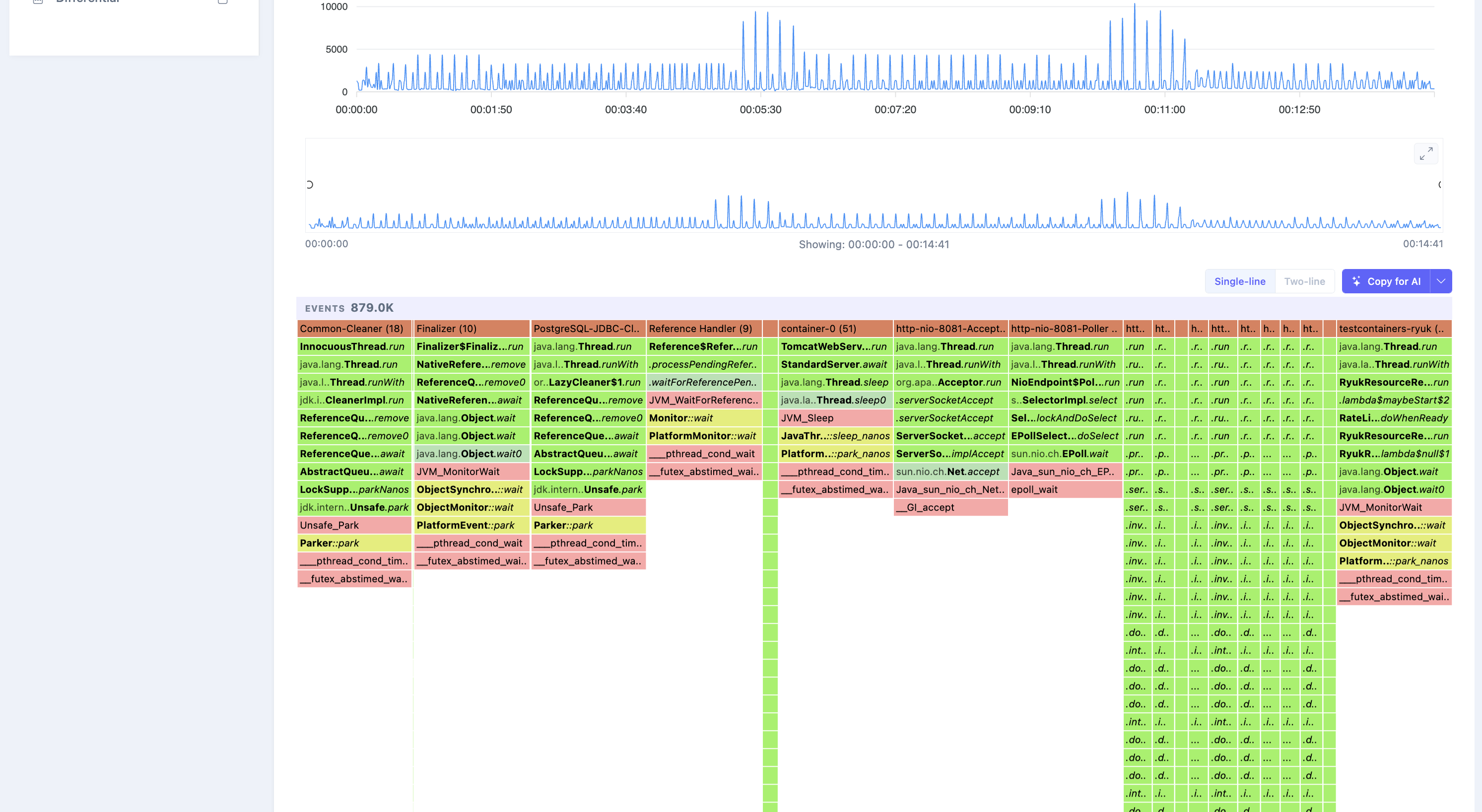
• Use Total Allocation – switches the allocation graph from sample count to weight: each frame is sized by the number of bytes allocated rather than how many samples hit it, so a rarely-sampled path that allocates large objects shows up at its true cost.

Weighting by the event's own measure instead of sample count often paints a very different — and more actionable — picture.

Summary

In this article, we set up Jeffrey Microscope and walked through reading a flamegraph — the timeseries and range selector, search, the frame tooltip, the Copy for AI export, and the allocation and wall-clock variants. That's already enough to find where an application spends its time and to start optimizing with confidence.

Thank you for reading! To go deeper, visit the Jeffrey pages, or reach out to me directly on LinkedIn — I'd love to hear your feedback. And stay tuned: in the next article, we'll put these two recordings side by side and show how Jeffrey's Differential flamegraph pinpoints exactly what changed between the optimized and unoptimized code.