Working With Time Series Data

According to DB-Engines, since 2016, time series has been the fastest growing database category. This popularity is fueled by the “sensorification” of the physical world (i.e., IoT) and the rapidly increasing instrumentation requirements of the next generation of software.

As we enter the era of workflow automation, machine learning and artificial intelligence, it is time for time series data.

A common question that comes to mind when the subject is times series data is: “What actually is it?” The more you think about it, the more you see it everywhere. Time is a constituent and inexorable part of everything that is observable. If it does not have a timestamp, it has no place in our universe. If time is always there as a dimension, time series means to treat every recorded data for what it is: unique. Therefore, it should not be replaced, but accumulated, appended as the next chapter in the “secret” time series life of the data.

Think of weather records showing that the Earth is getting warmer and ice caps are melting beyond historic limits. Or consider economic indicators showing how well a current administration is doing its job, such as changes in the GDP, income and wages, unemployment rate, inflation, etc. Other common examples include records of the evolving status of a patient under treatment, or tweets per hour for a specific hashtag, e.g. #royalbaby. The reality is that time series data is everywhere.

What classifies the data around you as time series depends on what it represents: a collection of measurements of the same thing over time, where you will find the time axis as you graph it. Bringing it to the tech world, time series are measurements that are tracked, monitored, downsampled and aggregated over time. This could be server metrics, application performance monitoring, network data, sensor data, events, clicks, trades in a market, and many other types of analytics data.

Time series:

Time Series Example: Stock Ticker Prices Over Time

Also time series:

So, what do time series give you besides a gigantic collection of data consuming your resources? If you can handle time series data properly, you can have application environments with close to zero-downtime, more and faster asset and resource consumption predictions using machine learning, workflow automation integrated with business KPIs, and ultimately, better customer experience leading to happier users.

Time series data personas are those responsible for maintaining a sustainable functional and evolving environment without operational downtime, inefficiencies and performance issues, while providing business units with means to monitor their own performance in order to stay on track of their goals. By doing so, time series personas provide the pillars for growth and success.

Time series projects usually start at DevOps and NetOps. They are the ones that must keep up with the speed of growth and complexity of the application environments, while coping with increasing intolerance to downtime or low performance. Monitoring production and pre-production as part of the application development lifecycle, as well as monitoring business performance indicators, is the way to detect trends early, anticipate resource requirements, and provide means to resolve issues in a timely manner.

Here are some case studies that illustrate specific scenarios where operational and business challenges can be addressed with the adoption of a time series platform solution.

SaaS companies looking for ensuring customer success find in time series a good strategy to achieve the ultimate goal of 100% uptime. They invest in DevOps monitoring solutions that provide visibility into performance, detecting early trends that could negatively impact the service. Monitoring is offered to the whole organization as a tool to assist teams (not just operations) to collect metrics that are relevant to them. Planning for scale, which includes not only being able to collect high volumes of data, but also automate the data life cycle while avoiding being locked in disparate systems is fundamental for a comprehensive approach.

E-commerce companies also rely on time series to keep user experience at its best. Ops monitoring teams work around the clock, 24x7, assuring the health of IT infrastructure and storefront applications. They integrate application monitoring as part of the application development process, so they come to production under the seal of “real user monitoring” (RUM) approval. For e-commerce companies with multiple data centers, handling volume and having HA becomes essential.

Companies that provide mobile services via smartphone applications are also benefiting from time series monitoring. Many of those companies have convenience and agility as core values. And although the service sometimes relies on a single smartphone app, the infrastructure and backend part of the application could be massive, with many components and microservices. As being fast, always ready, and at reach are all part of mobile services, they must detect problems before their users experience them. Once a user tries another service that works, this other service becomes the preferred choice. So, it is paramount to monitor metrics from systems, applications, and KPI at high sampling rates to catch anything that goes wrong practically as it happens. Certainly, the volume of data collected at rates of millions per second will be high, but as data gets cold, it could be aggregated for trending analysis. Therefore, beyond high volume and HA, the data life cycle is also fundamental for companies using time series monitoring to keep ahead of competition in the mobile applications market.

Cloud service providers also turn to multi-tenant metric-driven visibility to provide their customers with ways to monitor their applications environment, regardless if it runs on Kubernetes clusters, containers, virtual machines, bare metal, or a combination of these options – which is very probable. Regardless of the diversity of environments, everything needs to be ready and available from one data source. Collecting all metrics in one time series platform that can support multi-tenancy and HA is a necessary foundation for scalable cloud hosting services.

In the time of time series, professionals are getting insights on how change happens over time and ways to predict their course in the future while monitoring the present. But in order to leverage the benefits of time series to its full extent, it is necessary to be able to collect, store, and analyze data in real-time and at scale.

Open source means, among other things, free to use, but, most importantly, it means that ideas and information are shared openly and the community is encouraged to collaborate transparently. Every breakthrough is celebrated by all and takes everyone one step ahead, driving innovation at a much faster pace. Because of the many eyes and brains continuously testing and applying it in different use cases, open source is more reliable and secure.

In complex environments, open source provides the necessary freedom to adapt. With more shared code, APIs, plugins, and custom scripts, the community helps you to implement solutions that fit with your legacy applications and future choices, giving you more bandwidth to concentrate on delivering the business logic for your specific use cases.

The power of the open source community to drive innovation is unsurpassed by any proprietary software solutions because it is not about license, it is about collaboration that makes the whole greater than the sum of its parts, and transparency, where nothing is hidden, giving you a chance to make educated decisions. Open source also keeps your options open by avoiding vendor lock-in.

Time series data platforms pose intrinsic challenges in scalability, high availability, and usability when professionals try to use legacy database and query engine models. Addressing these challenges properly led to the development of time series databases. Those embarking on time series data projects face a major decision: try to adapt an existing relational database to manage times series data, or adopt time series databases with purpose-built storage and query engines?

Purpose-built time series database engines reach benchmarks in the order of hundreds of millions of time series, millions of writes per second, and over thousands of queries per second. Time series databases have a few properties that make them very different than other data stores: automated data lifecycle management, summarization, continuous queries, and large range scans of many records. There is still, of course, the obvious differentiation of having a time dimension present in everything done with the data: collecting, storing, replicating, querying, transforming, and evicting.

Although time must be a central point in the overall platform architecture design of the database, just being able to query on time doesn’t cover all the requirements of an effective and efficient solution. To achieve the envisioned scalability and usability paradigm of a very large and granular data set, it is necessary to devise a combined strategy in data model and storage engine design. Add to that a query language that eases selection of series, continuous queries, and transformation of queried data, and you have a complete time series platform, such as InfluxData’s TICK Stack.

InfluxData is an open source, purpose-built full-stack time series platform for managing time series data. We’ll begin by explaining each component that comprises the platform before moving into examples of how it can be used with time series data.

The functional architecture consists of four components — Telegraf, InfluxDB, Chronograf, and Kapacitor (TICK Stack). These components are built as an end-to-end solution for time series data use cases. Telegraf is built for data collection; InfluxDB is the database and storage tier; Chronograf is for visualization; and Kapacitor is the rules engine for processing, monitoring, and alerting. InfluxDB is a key component in the time series data platform architecture because it is designed to take the peculiar characteristics of time series data as insights to better handle it, in contrast to legacy storage engines and databases designs that only try to work around them, leading to limitations and performance issues.

InfluxDB Data Model Design

Efficiency and effectiveness have to start in the data structure, ensuring that time-stamped values are collected with the necessary precision and metadata to provide flexibility and speed in graphing, querying, and alerting. The InfluxDB data model has a flexible schema that accommodates the needs of diverse time series use cases. The data format takes the following form:

<measurement name>,<tag set> <field set> <timestamp>

The measurement name is a string, the tag set is a collection of key/value pairs where all values

are strings, and the field set is a collection of key/value pairs where the values can be int64, float64, bool, or string. There are no hard limits on the number of tags and fields.

Being able to have multiple fields and multiple tags under the same measurement optimizes the transmission of the data, avoiding multiple retransmissions which can render network protocols bloated when transmitting data with shared tag sets. This design choice is also particularly important for IoT use cases where the agent stored on the monitored remote devices sending the metrics has to be energy-efficient for longer lifespan.

Furthermore, support for multiple types of data encoding beyond float64 values means that metadata can be collected along with the time series, and not limited to monitor only numeric values. Precision is another parameter that must be taken into account when defining the data model. Timestamps in InfluxDB can be second, millisecond, microsecond, or nanosecond precision.

The measurement name and tag sets are kept in an inverted index which make lookups for specific series very fast.

See below CPU metrics mapped in InfluxDB line-protocol:

  cpu,host=serverA,region=uswest idle=23,user=42,system=12 1464623548s

InfluxDB Time Series Database Specialties

A good strategy when adopting a platform for time series should take into account the management of all types of time series data — not only metrics (numeric values regularly collected or pulled), but also events (pushed at irregular time intervals) such as faults, peaks, and human-triggered ones, such as clicks).

Since we are talking about a constant influx of granular data from a number of data sources, a performant database solution for time series has to handle high write rates with fast queries at scale, and that is where most other types of databases stumble when used for time series. In order to reach the bar lifted by time series, InfluxData implemented an architecture design with high compression, super-fast storage and query engines, and a purpose-built stack.

InfluxDB uses an append-only file for new data arrival in order to make new points quickly ingested and durable; a columnar on-disk storage for efficient queries and aggregations over time; a time- bound file structure that facilitates management of data in shards’ sizes; a reverse index mapping measurements to tags, fields and series, for quick access to targeted data; and data compaction and compression for read optimization and volume control.

InfluxDB was also designed to provide ease and automated data lifecycle management: retention policies, sharding, replication, and rollup capabilities built-in. In time series it’s common to keep high-precision data around for a short period of time, and then aggregate and downsample into longer-term trend data. This kind of data lifecycle management is difficult for application developers to implement on top of regular databases, but fundamental for time series.

The easiest way to get a feel for what time series data can do for you is to try it. Since the TICK Stack is open source, you can freely ,download and install Telegraf, InfluxDB, Chronograf and Kapacitor. Let’s start with InfluxDB, feed some data, and build some queries.

With InfluxDB installed, it is time to interact with the database. Let’s use the command line interface (influx) to write data manually, query that data interactively, and view query output in different formats. To access the CLI, first launch the influxd database process and then launch influx in your terminal. Once you’ve connected to an InfluxDB node, you’ll see the following output:

$influx                                                              

Connected to                                                          
[[http://localhost:8086]{.underline}](http://localhost:8086) version  
1.7x                                                                  

InfluxDB shell version 1.7.x                                          

Note that the version of InfluxDB and CLI must be identical.

Creating a Database in InfluxDB

A fresh install of InfluxDB has no databases (apart from the system _internal). You can create a database with the CREATE DATABASE <db-name> InfluxQL statement, where <db-name> is the name of the database you wish to create. Let’s create a database called mydb.

  > CREATE DATABASE mydb

To see if the database was created, use the following statement:

> SHOW DATABASES 

name: databases   

Name              

 ----           

_internal        

mydb              

Now, it is time to populate the mydb database.

Writing and Querying the Database

InfluxDB is populated with points from popular clients via HTTP /write Endpoint POST or via the CLI. Datapoints can be inserted individually or in batches.

Points consist of a timestamp, a measurement (“cpu_load”, for example), at least one key-value field (the measured value itself, e.g. “value=0.64”, or “temperature=21.2”), and zero to many key-value tags containing any metadata about the value (e.g. “host=server01”, “region=EMEA”, “dc=Frankfurt”).

Conceptually, you can think of a measurement as an SQL table, where the primary index is always time. Tags and fields are effectively columns in the table. Tags are indexed, and fields are not.

Points are written to InfluxDB using line protocol:

<measurement>[,<tag-key>=<tag-value>...] <field-key>=<field-value>[,<field2-key>=<field2-value>...] [unix-nano-timestamp]

To insert a single time series datapoint with the measurement name of cpu and tags host and region, with the measured value of 0.64 into InfluxDB using the CLI, enter INSERT followed by a point in line protocol format:

> INSERT cpu,host=serverA,region=us_west value=0.64

Now query for the data written:

> SELECT “host”, “region”, “value” FROM “cpu”
Name: cpu
---------
Time                           host    region  value
2015-10-21T19:28:07.5806643472 serverA us_west 0.64

Great! You successfully installed InfluxDB and can write and query the data.

Next step is to collect data via Telegraf and send it to InfluxDB.

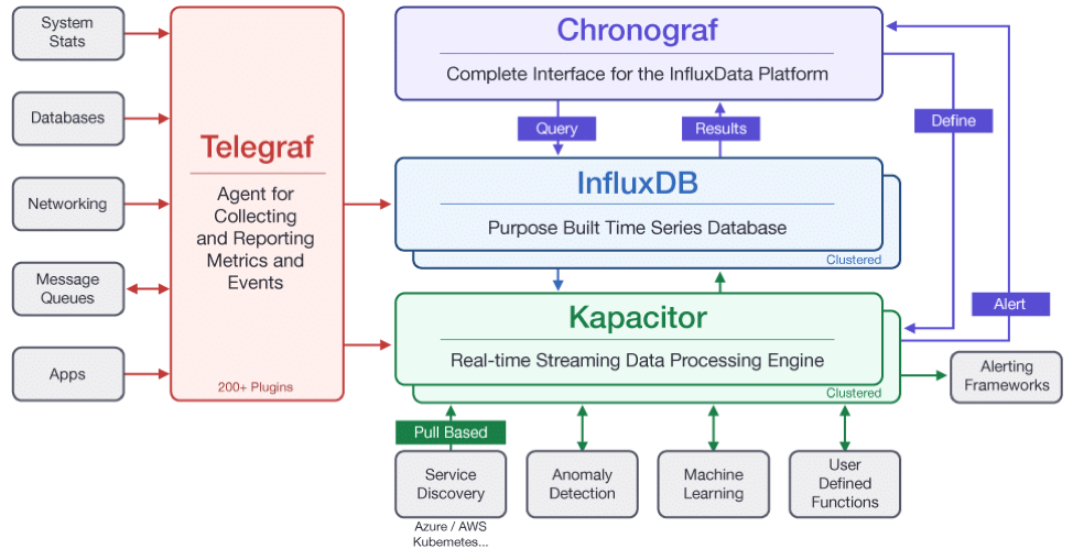
Data Collection with Telegraf

Telegraf is a plugin-driven server agent for collecting and reporting metrics. Telegraf has plugins to pull metrics from third-party APIs, or to listen for metrics via StatsD and Kafka consumer services. It also has output plugins to send metrics to a variety of datastores.

Install Telegraf from InfluxData download page: https://portal.influxdata.com/downloads/

Before starting the Telegraf server, you need to edit and/or create an initial configuration that specifies your desired inputs (where the metrics come from) and outputs (where the metrics go). Telegraf can collect data from the system it is running on. That is just what is needed to start getting familiar with Telegraf.

The example below shows how to create a configuration file called telegraf.conf with two inputs:

1. One input reads metrics about the system’s cpu usage (cpu).
2. Another input reads metrics about the system’s memory usage (mem).

InfluxDB is defined as the desired output.

telegraf -sample-config -input-filter cpu:mem -output-filter influxdb > telegraf.conf

Start the Telegraf service and direct it to the relevant configuration file:

MacOS Homebrew

telegraf -config telegraf.conf

Linux (sysvinit and upstart Installations)

Sudo services telegraf start

Linux (systemd Installations)

Systemctl start telegraf

You will see the following output (Note: this output below runs on a Mac):

NetOps-MacBook-Air:~ Admin$ telegraf --config telegraf.conf
2019-01-12T18:49:48Z I! Starting Telegraf 1.8.3
2019-01-12T18:49:48Z I! Loaded inputs: inputs.cpu inputs.mem
2019-01-12T18:49:48Z I! Loaded aggregators:
2019-01-12T18:49:48Z I! Loaded processors:
2019-01-12T18:49:48Z I! Loaded outputs: influxdb
2019-01-12T18:49:48Z I! Tags enabled: host=NetOps-MacBook-Air.local
2019-01-12T18:49:48Z I! Agent Config: Interval:10s, Quiet:false, Hostname:”NetOps-MacBook-Air.local”, Flush Internal:10s

Once Telegraf is up and running, it will start collecting data and writing it to the desired output.

Returning to our sample configuration, we show what the cpu and mem data look like in InfluxDB below. Note that we used the default input and output configuration settings to get this data.

List all measurements in the Telegraf database:

> SHOW MEASUREMENTS
Name: measurements
------------------
Name
Cpu
mem

List all field keys by measurement:

> SHOW FIELD KEYS
name: cpu
---------
fieldKey                fieldType
usage_guest             float
usage_guest_nice         float
usage_idle           float
usage_iowait             float
usage_irq            float
usage_nice           float
usage_softirq        float
usage_steal          float
usage_system             float
usage_user           float

name: mem
---------
fieldKey                fieldType
active               integer
available            integer
available_percent        float
buffered             integer
cached               integer
free                 integer
inactive             integer
total                  integer
used                   integer
used_percent               float

Select a sample of the data in the field usage_idle in the measurement cpu_usage_idle:

> SELECT usage_idle FROM cpu WHERE cpu = 'cpu-total' LIMIT 5
name: cpu
---------
time                           usage_idle
2016-01-16T00:03:00Z     97.56189047261816
2016-01-16T00:03:10Z     97.76305923519121
2016-01-16T00:03:20Z     97.32533433320835
2016-01-16T00:03:30Z     95.68857785553611
2016-01-16T00:03:40Z     98.63715928982245

That’s it! You now have the foundation for using Telegraf to collect and write metrics to your database.

Data visualization and graphing with Chronograf

Chronograf is the administrative interface and visualization engine for the TICK Stack. It is simple to use and includes templates and libraries to allow you to build dashboards of your data and to create alerting and automation rules.

The Chronograf builds are available on InfluxData’s Downloads page.

1. Choose the download link for your operating system.

Note: If your download includes a TAR package, we recommend specifying a location for the underlying datastore, chronograf-v1.db, outside of the directory from which you start Chronograf. This allows you to preserve and reference your existing datastore, including configurations and dashboards, when you download future versions.

2. Install Chronograf:

• MacOS: tar zxvf chronograf-1.6.2_darwin_amd64.tar.gz
• Ubuntu & Debian: sudo dpkg -i chronograf_1.6.2_amd64.deb
• RedHat and CentOS: sudo yum localinstall > chronograf-1.6.2.x86_64.rpm

3. Start Chronograf:

• MacOS: tar zxvf chronograf-1.6.2_darwin_amd64.tar.gz
• Ubuntu & Debian: sudo dpkg -i chronograf_1.6.2_amd64.deb

4. Connect Chronograf to your InfluxDB instance or InfluxDB Enterprise cluster:

• Point your web browser to > localhost:8888.
• Fill out the form with the following details:
  1. Connection String: Enter the hostname or IP of the machine that InfluxDB is running on, and be sure to include InfluxDB’s default port 8086.
  2. Connection Name: Enter a name for your connection string.
  3. Username and Password: These fields can remain blank unless you’ve enabled authorization in InfluxDB.
  4. Telegraf Database Name: Optionally, enter a name for your Telegraf database. The default name is Telegraf.
• Click Add Source.

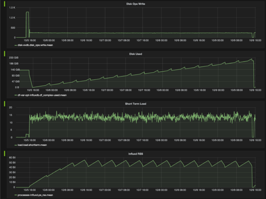
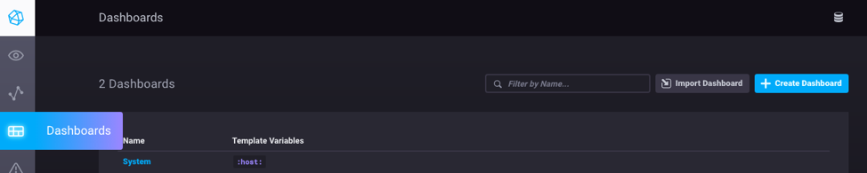
Pre-canned Dashboards

Pre-created dashboards are delivered with Chronograf, and you just have to enable the respective desired Telegraf plugins. In our example, we already enabled the cpu and mem plugins at the config file creation. Let’s take a look (Note: this example runs on a Mac):

Select the Dashboard icon in the navigation bar on the left, and then select “System”:

Voilà!

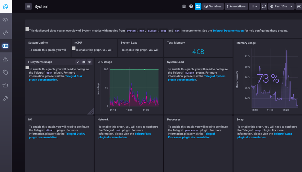
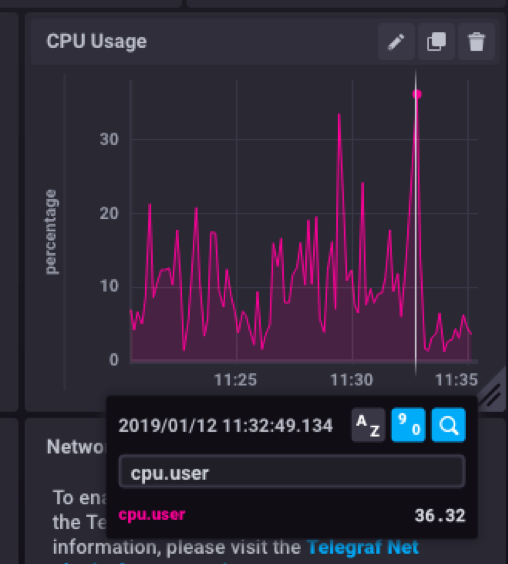
Taking a closer look at cpu measurement, you can see that it shows three measured fields (cpu.idle, cpu.user and cpu.system). You can filter each and move the measurement line to show exact values and timestamp.

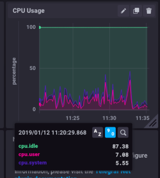
Cpu.user metric filtered:

The selected "System" App option for the example is just one of many pre-created dashboards available in Chronograf. See the list below:

• apache
• consul
• docker
• elasticsearch
• haproxy
• iis
• influxdb
• kubernetes
• memcached
• mesos
• mysql
• nginx
• nsq
• phpfpm
• ping
• postgresql
• rabbitmq
• redis
• riak
• system
• varnish
• win_system

Now that you are set to start exploring the world of time series data, what is next? Learning from others experience is always a good idea. Get more insights from case studies in various industry segments: telecom and service providers, e-commerce, financial markets, IoT, research, manufacturing, telemetry, and of course, the horizontal case of DevOps and NetOps in any organization, and see how time series monitoring generated positive results in the organizations, from better resource management via automation and prediction to five star customer experience.