Building Neural Networks With Automatic Differentiation

One of the biggest reasons for the fast pace of research and progress in modern AI is due to the availability of Python libraries such as PyTorch, TensorFlow, and JAX. Python itself is considered one of the easiest programming languages to pick up, and these ML/DeepLearning libraries make prototyping and testing sophisticated ML models much more accessible to engineers, researchers, and even enthusiasts.

One key idea that has driven tremendous success in training large ML and neural network models is automatic differentiation (AD). It is the mechanism that enables backpropagation in neural networks. The main idea behind AD is to recursively calculate the partial derivatives (using the chain rule) for a neural network, which is represented as a directed acyclic graph (DAG). It’s a simple technique but very powerful. 

In this post, we are going to write our own simple neural network from scratch and train it with gradient backpropagation while using only basic Python libraries. I hope this not only demystifies the idea of automatic differentiation and lets you appreciate the power of a simple technique but also elevates your understanding of some of the ideas and techniques utilized in writing deep-learning libraries.

Today, 70% of the users prefer to use Pytorch over Tensorflow. Tensorflow used to be the library of choice for both academia/research and industry till a few years ago, but Pytorch won that race and is by far the favored choice now. Arguably, the biggest reason for that switch is that unlike Tensorflow and JAX, which use a static computation graph, Pytorch uses a dynamic computation graph. This makes it much easier and intuitive to use as the API and operations integrate seamlessly with Python workflows, and that's the model we will follow to build our neural network from scratch.

Automatic Differentiation

Let’s start with a very simple expression:

y = a*x + b 

If we differentiate f(x) = y with respect to 'x,' we get 'a.' We have two goals:

• Write the equation for f(x) in Python, hopefully like a graph
• Backpropagate on that graph eg. to estimate 'a' and 'b' given multiple values of 'x' and 'y'

There's no direct way to write mathematical expressions in Python, so we need to define some sort of abstraction/class/object that we can use to represent each of the items 'y,' 'a,' 'x,' and 'b' and we want that object to be able to do the following:

1. Hold a value
2. Support operations on it, such as multiplication, addition, etc.

To that end, let's create a Node class that can do those things. The reason for naming it should become clearer later on.

class Node(object):
  
  def __init__(self, value):
    self.value = value
    
  def __add__(self, other):
    if isinstance(other, (int, float)):
      '''
      So we can add ints and floats directly to a Node
      '''
      other = Node(other)
     
    if not isinstance(other, Node):
      raise ValueError(f"Unknown type: {type(other)} being added to Node")
     
    new_node = Node(self.value + other.value)
    return new_node
  
  def __radd__(self, other):
    '''
    Take care of situation when item on the left side of the operation
    is not of type Node. 
    '''
    return self.__add(other)
  
  def __mul__(self, other):
    if isinstance(other, (int, float)):
      other = Node(other)
    
    if not isinstance(other, Node):
      raise ValueError(f"Unknown type: {type(other)} being added to Node")
     
    new_node = Node(self.value * other.value)
    return new_node
   
  def __rmul__(self, other):
    return self.__mul__(other)
  
  def __str__(self, other):
    print(f'Node value is {self.value}')

There are a few things going on here, so let me explain.

• The __add__(...) method overloads the + operator on an object, allowing us to add two Node objects or a Node and a scalar (int/float).
• The __add__(...) only overloads the operator present on the right side of the operand, e.g., 'Node + ...'. It doesn't overload an operation as ... + Node. That's being done by __radd__(...), which is short for "right add," and that should explain why that's overloaded as well 
• The exact same thing is done for overloading the * operator using __mul__(...).
• The __str__ defines the string representation on an object (useful for printing).

Just with this definition, we can write code such as:

a = Node(3)
y = a*2 + 1
print(y)

>>> Node value is 7

In the code above, x = 2, a = 3, b = 1 and f(x) = y = 7.

The next step is to figure out how to compute the derivative, e.g., δf(x)/δx above in software. Here's another example, with the relevant derivatives computed using the chain rule:

x1 = Node(1)
x2 = Node(2)
x3 = x1 + x2
x4 = Node(3)
x5 = x3 * x4

δx5/δx4 = x3
δx5/δx3 = x4

-- Using Chain Rule
δx5/δx1 = δx5/δx3 * δx3/δx1 = x4 * 2
δx5/δx2 = δx5/δx3 * δx3/δx2 = x4 * 3

Now, what we want our code to do is compute δx5/δx1 and set an attribute for x1 Node object with that value. To explain how we will accomplish that, I am going to define a few things first:

• Child Node – Node that has an operand (e.g. + or *) applied to it to generate a new node. x1, x2, x3, and x4 are all child nodes. 
• Parent Node – Result of an operation on two or more nodes. x3 and x5 are parent nodes. Note that a node can be both a parent and a child.
• Node Gradient – Gradient of a 'child' node with respect to a 'parent' node.
  **Assumption: We will construct a sorted (topological) graph (DAG) and compute gradients starting from the very last node (the parent node with no parents of its own, only children) and ending at the very first node(the child node with only parents and no children).

Now, let's say that for a child node 'child,' we know the Node Gradient: δ(parent)/δ(child), then the gradient of 'child' with respect to any other node 'X' can be computed as: δ(X)/δ(parent) * δ(parent)/δ(child). If node 'X' comes before 'parent' in the topologically sorted graph and we are computing gradients in order, it's safe to assume that we would have already computed 'δ(X)/δ(parent).' So, all we need to know is δ(parent)/δ(child).

Based on the understanding so far, we can modify the __init__, __add__, and __mul__ methods as follows:

class Node(object):
    def __init__(self, value, children=None):
        self.value = value
        self.backward_grad = lambda: None # This method is called to calculate grad at each update
        self.grad = 0 # Stores the computed gradient to be used by any children nodes and to update value
        self.children = children # We store children so we can construct a topologically sorted graph when doing backprop
        
    def __add__(self, other):
        if isinstance(other, (int, float)):
            other = Node(other)
        
        if not isinstance(other, Node):
            raise TypeError(f'Unknown type: {type(other)} being added to Node')

        parent = Node(self.value + other.value, [self, other])

        '''
        The following is a python closure, and it stores references to self, other and parent.
        This is similar to the concept of a lambda function in C++, which is actually a class 
        with a single operator() method and it stores references to anything that's captured 
        NOTE: 'self.grad += ...' NOT 'self.grad = ...' . The reason for this would become clear
        later 
        '''
        def backward():
            self.grad += parent.grad * 1.0 # Under simple addition δ(parent)/δ(self) is just 1
            other.grad += parent.grad * 1.0 # Under simple addition δ(parent)/δ(other) is just 1
		'''
        There's an argument to be made that, why not reset the backward_grad method for 
        'self' and 'other' instead of 'parent'. The reason is that it becomes tricky to handle in
        cases where self and other are the same node. This is much cleaner. 
        '''
        parent.backward_grad = backward       
        return parent
      
    def __mul__(self, other):
        if isinstance(other, (int, float)):
            other = Node(other)

        if not isinstance(other, Node):
            raise TypeError(f'Unknown type: {type(other)} being multiplied to Node')
        
        parent = Node(self.value * other.value, [self, other])

        def backward():
            self.grad += parent.grad * other.value # Under multiplication δ(parent)/δ(self) is other
            other.grad += parent.grad * self.value # Under multiplication δ(parent)/δ(other) is self
        
        parent.backward_grad = backward
        return parent

If you check the code we have written above, these are exactly the values we will get. I leave it as an exercise for the reader to verify. This computation of the partial gradient of nodes in a graph algorithmically or automatically using a program is what's called automatic differentiation. 

There's only one thing remaining to make our Node class complete: a method to construct a graph (topologically sorted) and compute gradients for all the nodes in this graph. This method would be called on the output Node, as that's the first node, and the graph would be constructed by connecting the children for each node at each step.

    def calculate_gradient(self):
        # construct a topological graph from the last node and then compute the gradient 1by1
        # order of the graph should be the order in which gradient should be computed, so nodes
        # closer to the output come before the nodes further from the output
        def topological_sort(current_node, visited, output):
            for node in current_node.children:
                if node not in visited:
                    visited.add(node)
                    topological_sort(node, visited, output)
            output.append(current_node)
        graph = []
        topological_sort(self, set(), graph)

        for node in graph[::-1]:
            node.backward_grad()

You might have noticed a comment in the __add__ method earlier:

• NOTE: 'self.grad += ...' NOT 'self.grad = ...'

The reason is that a child node can feed into multiple parent nodes, for example:

c = a + b
d = a + e
z = d * c

In this case, node 'a' has two parents: 'd' and 'c.' The gradients from both of them should flow into 'a' and should be added. This comes from the chain rule under the multivariable case. To understand this intuitively, consider the most simple example:

b = a + a

δb/δa = 1 + 1 = 2

Let's test what we have talked so far with the following code:

def test_nodes():
    a = Node(4)
    b = Node(6)
    e = Node(2)
    c = a + b
    d = a + e
    z = d * c
    z.grad = 1.0
    z.calculate_gradient()
    
    print(f'a.grad: {a.grad}')
    print(f'b.grad: {b.grad}')
    print(f'c.grad: {c.grad}')
    print(f'd.grad: {d.grad}')
    print(f'e.grad: {e.grad}')

The code above prints:

a.grad: 16.0
b.grad: 6.0
c.grad: 6.0
d.grad: 10.0
e.grad: 10.0

This is exactly what we would expect! I leave it as an exercise for the reader to verify. 

Now, to be able to have non-linearity in our neural network, we need to add an activation function to our Node. I am going to add Tanh and ReLu. The former is because its output is (-1, 1), and the latter is because it's fairly easy to implement and works well. 

    def relu(self):
        parent = Node(0 if self.value < 0 else self.value, [self])

        def backward():
          '''
          No gradient update if the value is <= 0
          '''
            if self.value > 0 : 
                self.grad += parent.grad
        
        parent.backward_grad = backward

        return parent
    
    def tanh(self):
        e = math.exp(2*self.value)
        t = (e + (-1))/(e + 1)
        parent = Node(t, [self])

        # derivative for tanh is 1 - tanh^2
        # this is easy to prove by substituting y = (exp(2x) + 1)
        def backward():
            self.grad += (1-t**2) * parent.value

        parent.backward_grad = backward

        return parent

Multi-Layer Perceptron

Our Node class is complete now. We need two more small classes before we can create our very own MLP (multi-layer perceptron) that we can train. Here they are:

class Neuron(object):
    def __init__(self, input_size):
        self.weights = [Node(np.random.randn()) for _ in range(input_size)]
        self.bias = Node(np.random.randn())
    
    def __call__(self, x):
        return (sum([w*x for w, x in zip(self.weights, x)]) + self.bias).tanh()

class Layer(object):
    def __init__(self, input_size, output_size):
        self.neurons = [Neuron(input_size) for _ in range(output_size)]
    
    def __call__(self, x):
        return [neuron(x) for neuron in self.neurons]

Each 'Neuron' can take a single dimensional input vector of any size and output a scalar. Each 'Layer' can take multiple 'scalars' as input and generate multiple 'Neurons' as output. Next, an MLP is just some layers connected together:

class MLP(object):
    def __init__(self, input_dim, hidden_dims):
        self.layers = []
        dim1 = input_dim
        for dim in hidden_dims:
            self.layers.append(Layer(dim1, dim))
            dim1 = dim
    
    def __call__(self, x):
        for layer in self.layers:
            x = layer(x)
        return x

And that's it! We have completed our implementation of a neural network from scratch. Let's try to train this network on a toy dataset.

Training an MLP

Here are the steps needed to train any network:

• Infer on a batch of inputs
• Compute the deviation/loss compared to the labels
• Backpropagate to compute the gradients of all the parameters 
• Update the parameters

There are two things still missing from our MLP class to realize all the steps above. First, we need to be able to fetch all the parameters from an MLP. Let's add a method for that.

class Layer(object):
	...
    
    def get_params(self):
        return [p for neuron in self.neurons for p in neuron.get_params()]


class MLP(object):
    ...
    
    def get_params(self):
        return [p for layer in self.layers for p in layer.get_params()]

Second, before we compute the gradient, we need to reset/unset any past gradients that may have been computed and stored.

class MLP(object):
	...
    
    def reset_grad(self):
        for p in self.get_params():
            p.grad = 0

Now, we are ready to train our neural network. Here's a toy example along with the training loop:

def train_MLP():
    mlp = MLP(3, [4, 4, 1])
    Xs = [
        [2, 1, 0],
        [0, -1, 3],
        [0, .1, 0],
        [4, 0.2, 5]
    ]
    ys = [-1, 1, -1, 1]

    def get_loss():
        y_pred = [mlp(x)[0] for x in Xs]
        return sum(((y1-y2)*(y1-y2) for y1, y2 in zip(ys, y_pred)))

    learning_rate = 0.01
    for i in range(30):
        loss = get_loss()
        mlp.reset_grad()
        loss.grad = 1.0
        loss.calculate_gradient()
        for p in mlp.get_params():
            p.value -= learning_rate * p.grad
        print(f'loss: {loss}')

This prints the following:

loss: 7.940816679052144
loss: 7.920999749612354
loss: 7.864187280538216
loss: 7.672885799925796
loss: 7.447409168213748
loss: 7.180697308979655
loss: 6.6726111418826655
loss: 5.683534417249739
loss: 3.595511286581251
loss: 3.903005951701422
loss: 1.0356346463474488
loss: 0.22743560632086313
loss: 0.12415406229882148
...

This shows that the network learned to fit that data and our code works! We can also try on something a little more complicated, e.g., make_blobs or make_circles. 

Example code to train:

def train_MLP():
    mlp = MLP(2, [32, 32, 1])
    Xs, ys = make_blobs(n_samples=100, centers=2)
    ys = ys*2 - 1 # to convert 0, 1 -> -1, 1
    def get_loss():
        y_pred = [mlp(x)[0] for x in Xs]
        return sum((y1-float(y2)) * (y1-float(y2)) for y1, y2 in zip(y_pred, ys))
    
    learning_rate = 0.002
    for i in range(10):
        loss = get_loss()
        mlp.reset_grad()
        loss.grad = 1.0
        loss.calculate_gradient()
        for p in mlp.get_params():
            p.value -= learning_rate * p.grad
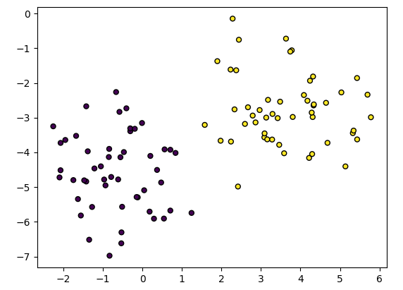
        print(f'loss: {loss}')

Just for your information, the blobs generated might look something like the following:

Running the training loop prints the following:

loss: 376.2473632585217
loss: 260.6936514763937
loss: 229.79644114625324
loss: 143.82531957969715
loss: 88.14959923975324
loss: 0.3732263521409278
loss: 0.06391714523542179
loss: 0.041553702053845794
loss: 0.03121547009281153
.... 

There it is. We have written a neural network from scratch that can be trained and used. It may be clear by this point that the MLP we have built is almost as powerful as the one implemented in Pytorch. This can be further expanded to build more complicated structures, e.g., adding other activation functions, operations such as 'exponent' or 'divide,' or even writing a CNN using Nodes as elements of a kernel.

Here's the complete code for your reference.