Computer Vision Tutorial 2: Image Basics

This tutorial is the foundation of computer vision delivered as “Lesson 2” of the series; there are more lessons upcoming that will talk to the extent of building your own deep learning-based computer vision projects. You can find the complete syllabus and table of contents here.

The main takeaways from this article:

• Loading an Image from Disk.
• Obtaining the ‘Height,’ ‘Width,’ and ‘Depth’ of the Image.
• Finding R, G, and B components of the Image.
• Drawing using OpenCV.

Loading an Image From Disk

Before we perform any operations or manipulations of an image, it is important for us to load an image of our choice to the disk. We will perform this activity using OpenCV. There are two ways we can perform this loading operation. One way is to load the image by simply passing the image path and image file to the OpenCV’s “imread” function. The other way is to pass the image through a command line argument using python module argparse.

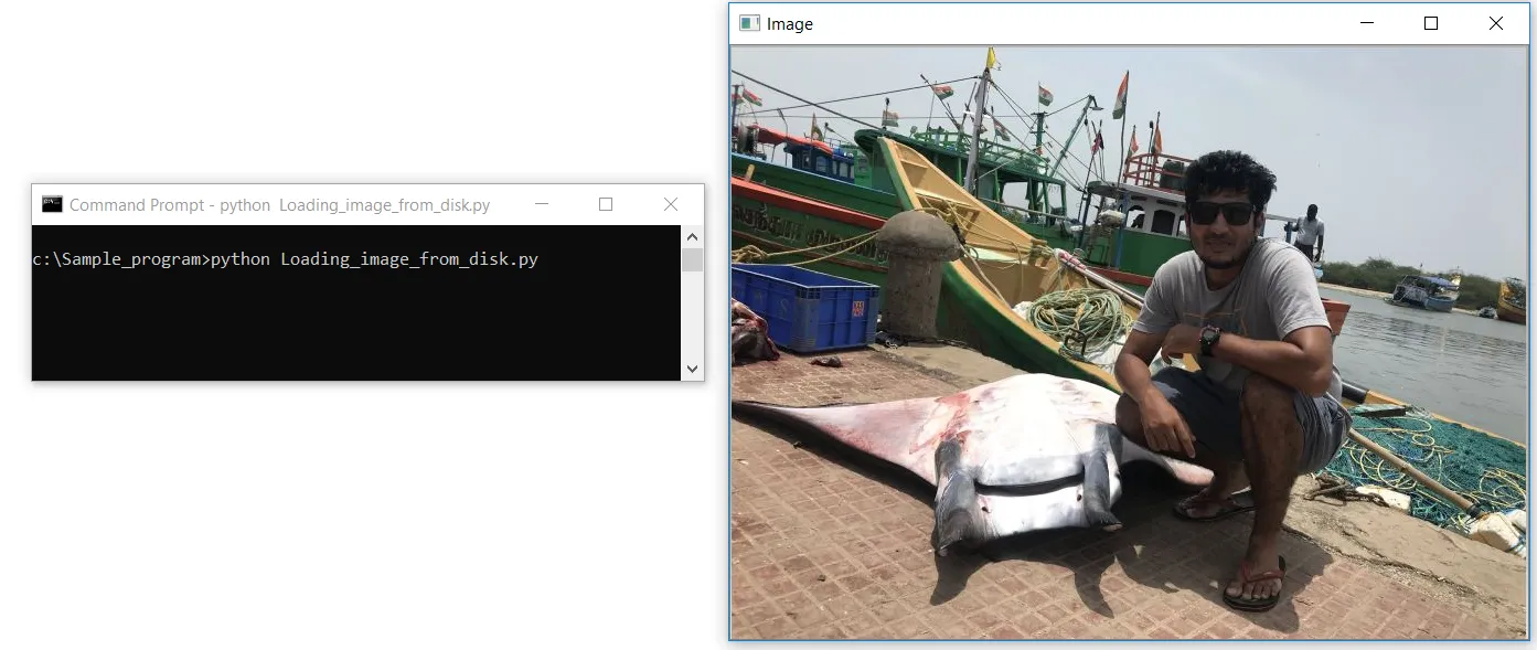
#Loading Image from disk

import cv2
image = cv2.imread(“C:/Sample_program/example.jpg”)
cv2.imshow(‘Image’, image)
cv2.waitKey(0)

Let’s create a file name Loading_image_from_disk.py in a notepad++. First, we import our OpenCV library, which contains our image-processing functions. We import the library using the first line of code as cv2. The second line of code is where we read our image using the cv2.imread function in OpenCV, and we pass on the path of the image as a parameter; the path should also contain the file name with its image format extension .jpg, .jpeg, .png, or .tiff.

syntax — // image=cv2.imread(“path/to/your/image.jpg”) //

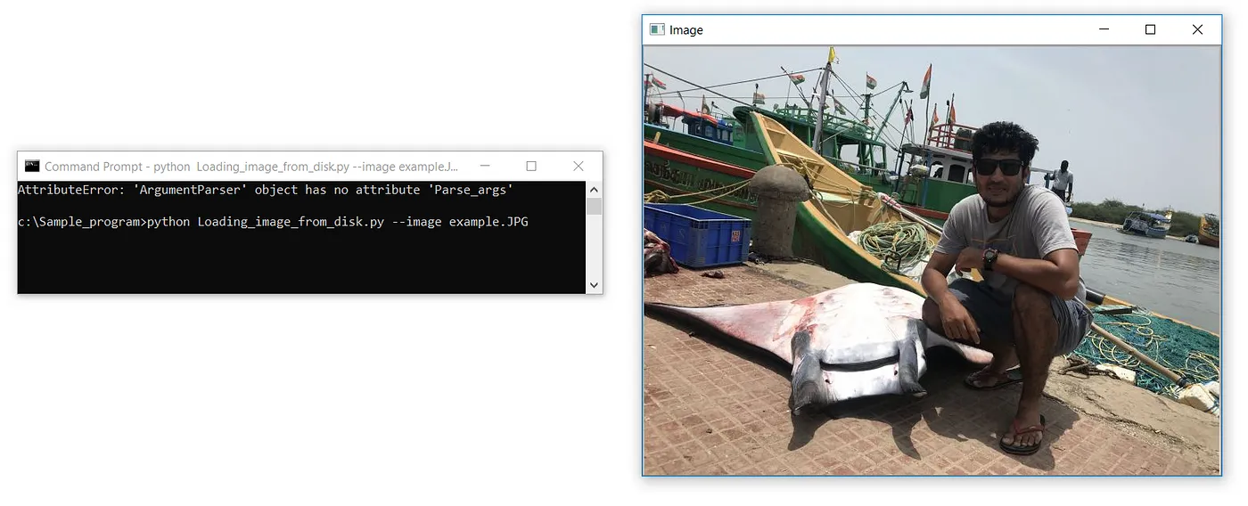
Absolute care has to be taken while specifying the file extension name. We are likely to receive the below error if we provide the wrong extension name.

ERROR :

c:\Sample_program>python Loading_image_from_disk.py
Traceback (most recent call last):
File “Loading_image_from_disk.py”, line 4, in <module>
cv2.imshow(‘Image’, image)
cv2.error: OpenCV(4.3.0) C:\projects\opencv-python\opencv\modules\highgui\src\window.cpp:376: error: (-215:Assertion failed) size.width>0 && size.height>0 in function ‘cv::imshow’

The third line of code is where we actually display our image loaded. The first parameter is a string, or the “name” of our window. The second parameter is the object to which the image was loaded.

Finally, a call to cv2.waitKey pauses the execution of the script until we press a key on our keyboard. Using a parameter of “0” indicates that any keypress will un-pause the execution. Please feel free to run your program without having the last line of code in your program to see the difference.

#Reading Image from disk using Argparse

import cv2
import argparse

apr = argparse.ArgumentParser()
apr.add_argument(“-i”, “ — image”, required=True, help=”Path to the image”)
args = vars(apr.parse_args())

image = cv2.imread(args[“image”])
cv2.imshow(‘Image’, image)
cv2.waitKey(0)

Knowing to read an image or file using a command line argument (argparse) is an absolutely necessary skill.

The first two lines of code are to import necessary libraries; here, we import OpenCV and Argparse. We will be repeating this throughout the course.

The following three lines of code handle parsing the command line arguments. The only argument we need is — image: the path to our image on disk. Finally, we parse the arguments and store them in a dictionary called args.

Let’s take a second and quickly discuss exactly what the — image switch is. The — image “switch” (“switch” is a synonym for “command line argument” and the terms can be used interchangeably) is a string that we specify at the command line. This switch tells our Loading_image_from_disk.py script, where the image we want to load lives on disk.

The last three lines of code are discussed earlier; the cv2.imread function takes args[“image’] as a parameter, which is nothing but the image we provide in the command prompt. cv2.imshow displays the image, which is already stored in an image object from the previous line. The last line pauses the execution of the script until we press a key on our keyboard.

One of the major advantages of using an argparse — command line argument is that we will be able to load images from different folder locations without having to change the image path in our program by dynamically passing the image path Ex — “ C:\CV_Material\image\sample.jpg “ in the command prompt as an argument while we execute our python program.

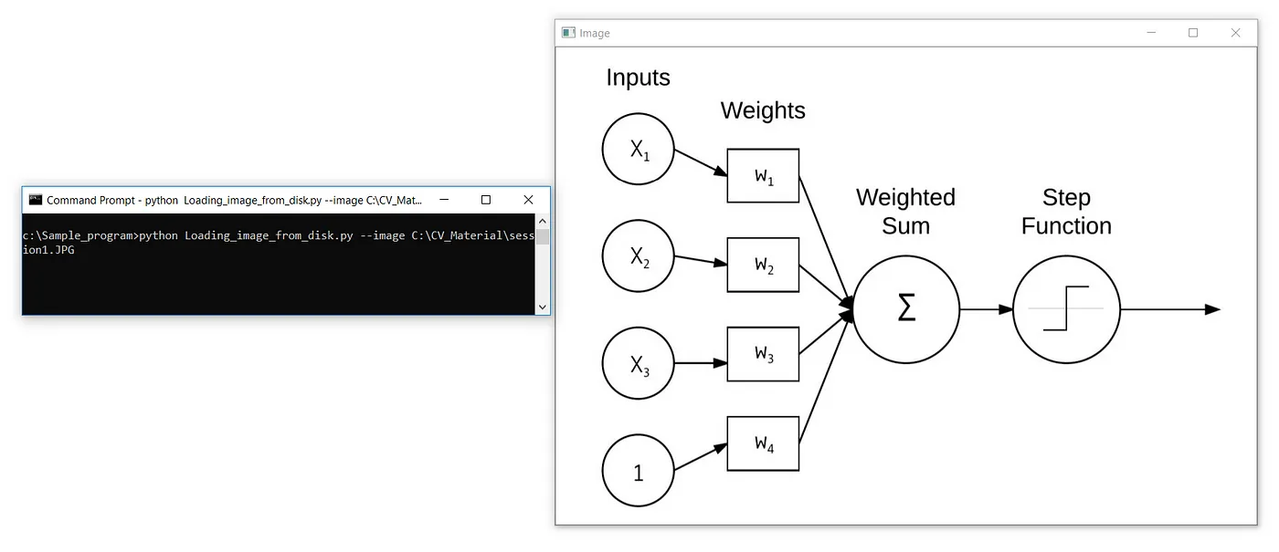
c:\Sample_program>python Loading_image_from_disk.py — image C:\CV_Material\session1.JPG

Here, we are executing the Loading_image_from_disk.py python file from c:\sample_program location by passing the “-image” parameter along with the path of image C:\CV_Material\session1.JPG.

Obtaining the ‘Height’, ‘Width’ and ‘Depth’ of Image

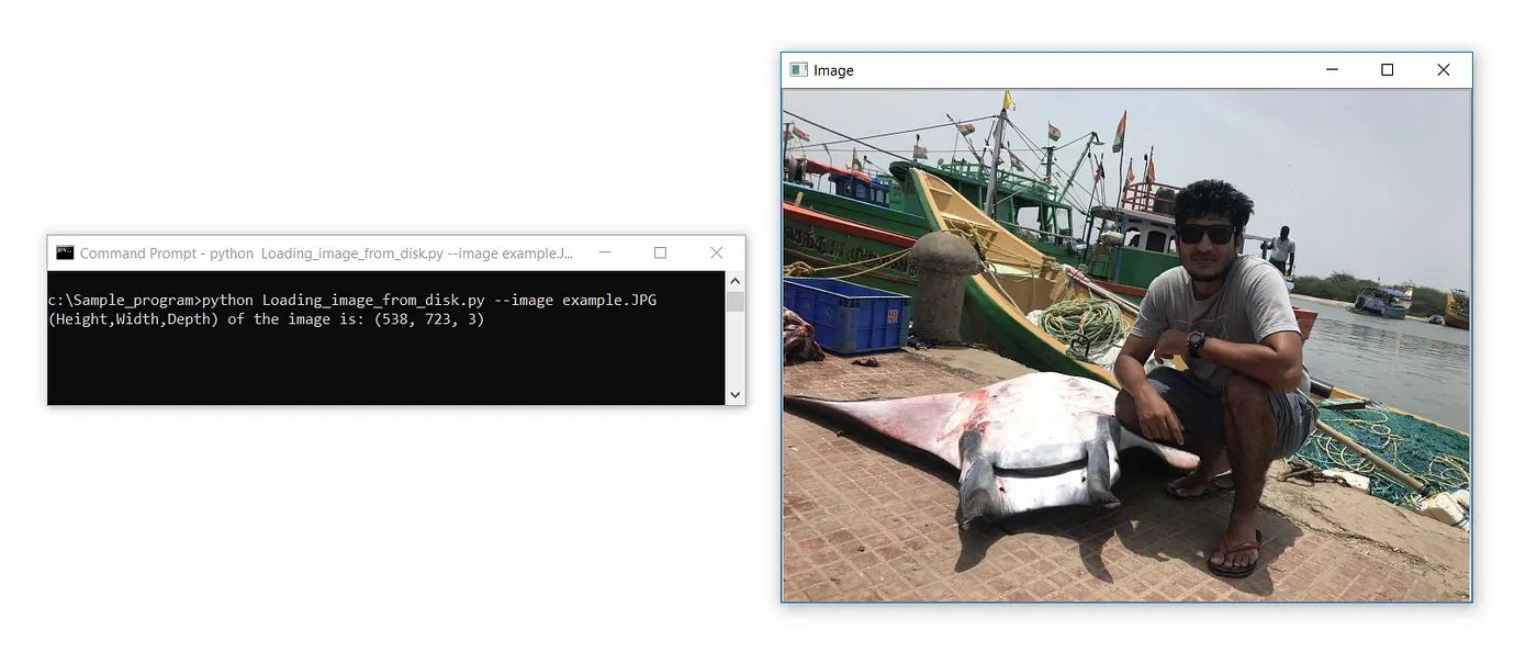
Since images are represented as NumPy arrays, we can simply use the .shape attribute to examine the width, height, and number of channels.

By using the .shape attribute on the image object we just loaded. We can find the height, Width, and Depth of the image. As discussed in the previous lesson — 1, the Height and width of the image can be cross-verified by opening the image in MS Paint. Refer to the previous lesson. We will discuss about the depth of image in the upcoming lessons. Depth is also known as channel of an image. Colored images are usually of 3 channel because of the RGB composition in its pixels and grey scaled images are of 1 channel. This is something we had discussed in the previous Lesson-1.

#Obtaining Height,Width and Depth of an Image

import cv2
import argparse

apr = argparse.ArgumentParser()
apr.add_argument(“-i”, “ — image”, required=True, help=”Path to the image”)
args = vars(apr.parse_args())

# Only difference to the previous codes — shape attribute applied on image object

print(f’(Height,Width,Depth) of the image is: {image.shape}’)

image = cv2.imread(args[“image”])
cv2.imshow(‘Image’, image)
cv2.waitKey(0)

Output:

(Height, Width, Depth) of the image is: (538, 723, 3)

The only difference from the previous codes is the print statement that applies the shape attribute to the loaded image object. f’ is the F-string @ formatted string that takes variables dynamically and prints.

f’ write anything here that you want to see in the print statement: {variables, variables, object, object.attribute,}’

Here, we have used {object.attribute} inside the flower bracket for the .shape attribute to compute the image object's height, width, and depth.

#Obtaining Height,Width and Depth separately

import cv2
import argparse

apr = argparse.ArgumentParser()
apr.add_argument(“-i”, “ — image”, required=True, help=”Path to the image”)
args = vars(apr.parse_args())

image = cv2.imread(args[“image”])

# NumPy array slicing to obtain the height, width and depth separately

print(“height: %d pixels” % (image.shape[0]))
print(“width: %d pixels” % (image.shape[1]))
print(“depth: %d” % (image.shape[2]))

cv2.imshow(‘Image’, image)
cv2.waitKey(0)

Output:

width: 723 pixels
height: 538 pixels
depth: 3

Here, instead of obtaining the (height, width, and depth) together as a tuple. We perform array slicing and obtain the height, width, and depth of the image individually. The 0th index of array contains the height of the image, 1st index contains the image's width, and 2nd index contains the depth of the image.

Finding R, G, and B Components of the Image

Output:

The Blue Green Red component value of the image at position (321, 308) is: (238, 242, 253)

Notice how the y value is passed in before the x value — this syntax may feel counter-intuitive at first, but it is consistent with how we access values in a matrix: first we specify the row number, then the column number. From there, we are given a tuple representing the image's Blue, Green, and Red components.

We can also change the color of a pixel at a given position by reversing the operation.

#Finding R,B,G of the Image at (x,y) position

import cv2
import argparse

apr = argparse.ArgumentParser()
apr.add_argument(“-i”, “ — image”, required=True, help=”Path to the image”)
args = vars(apr.parse_args())

image = cv2.imread(args[“image”])

# Receive the pixel co-ordinate value as [y,x] from the user, for which the RGB values has to be computed
[y,x] = list(int(x.strip()) for x in input().split(‘,’))

# Extract the (Blue,green,red) values of the received pixel co-ordinate
(b,g,r) = image[y,x]
print(f’The Blue Green Red component value of the image at position {(y,x)} is: {(b,g,r)}’)

cv2.imshow(‘Image’, image)
cv2.waitKey(0)

(b,g,r) = image[y,x] to image[y,x] = (b,g,r)

Here we assign the color in (BGR) to the image pixel co-ordinate. Let's try by assigning RED color to the pixel at position (321,308) and validate the same by printing the pixel BGR at the given position.

#Reversing the Operation to assign RGB value to the pixel of our choice

import cv2
import argparse

apr = argparse.ArgumentParser()
apr.add_argument(“-i”, “ — image”, required=True, help=”Path to the image”)
args = vars(apr.parse_args())

image = cv2.imread(args[“image”])

# Receive the pixel co-ordinate value as [y,x] from the user, for which the RGB values has to be computed
[y,x] = list(int(x.strip()) for x in input().split(‘,’))

# Extract the (Blue,green,red) values of the received pixel co-ordinate
image[y,x] = (0,0,255)
(b,g,r) = image[y,x]
print(f’The Blue Green Red component value of the image at position {(y,x)} is: {(b,g,r)}’)

cv2.imshow(‘Image’, image)
cv2.waitKey(0)

Output:

The Blue, Green, and Red component values of the image at position (321, 308) are (0, 0, 255)

In the above code, we receive the pixel co-ordinate through the command prompt by entering the value as shown in the below Fig 2.6 and assign the pixel co-ordinate red color by assigning (0,0,255) ie,(Blue, Green, Red) and validate the same by printing the input pixel co-ordinate.

Drawing Using OpenCV

Let's learn how to draw different shapes like rectangles, squares, and circles using OpenCV by drawing circles to mask my eyes, rectangles to mask my lips, and rectangles to mask the mantra-ray fish next to me.

The output should look like this:

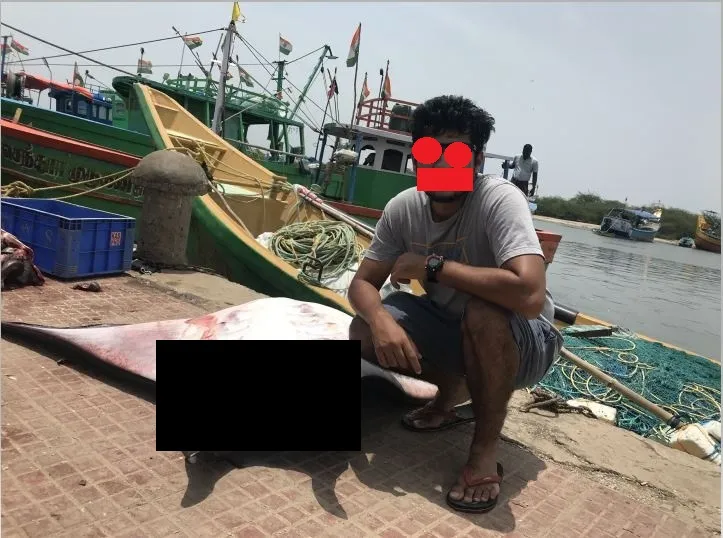
This photo is masked with shapes using MS Paint; we will try to do the same using OpenCV by drawing circles around my eyes and rectangles to mask my lips and the matra-ray fish next to me.

We use cv2.rectangle method to draw a rectangle and cv2.circle method to draw a circle in OpenCV.

cv2.rectangle(image, (x1, y1), (x2, y2), (Blue, Green, Red), Thickness)

The cv2.rectangle method takes an image as its first argument on which we want to draw our rectangle. We want to draw on the loaded image object, so we pass it into the method. The second argument is the starting (x1, y1) position of our rectangle — here, we are starting our rectangle at points (156 and 340). Then, we must provide an ending (x2, y2) point for the rectangle. We decide to end our rectangle at (360, 450). The following argument is the color of the rectangle we want to draw; here, in this case, we are passing black color in BGR format, i.e.,(0,0,0). Finally, the last argument we pass is the thickness of the line. We give -1 to draw solid shapes, as seen in Fig 2.6.

Similarly, we use cv2.circle method to draw the circle.

cv2.circle(image, (x, y), r, (Blue, Green, Red), Thickness)

The cv2.circle method takes an image as its first argument on which we want to draw our rectangle. We want to draw on the image object that we have loaded, so we pass it into the method. The second argument is the center (x, y) position of our circle — here, we have taken our circle at point (343, 243). The following argument is the radius of the circle we want to draw. The following argument is the color of the circle; here, in this case, we are passing RED color in BGR format, i.e.,(0,0,255). Finally, the last argument we pass is the thickness of the line. We give -1 to draw solid shapes, as seen in Fig 2.6.

Ok ! By knowing all this. Let's try to accomplish what we started. To draw the shapes in the image, we need to identify the masking region's starting and ending (x,y) coordinates to pass it to the respective method.

How?

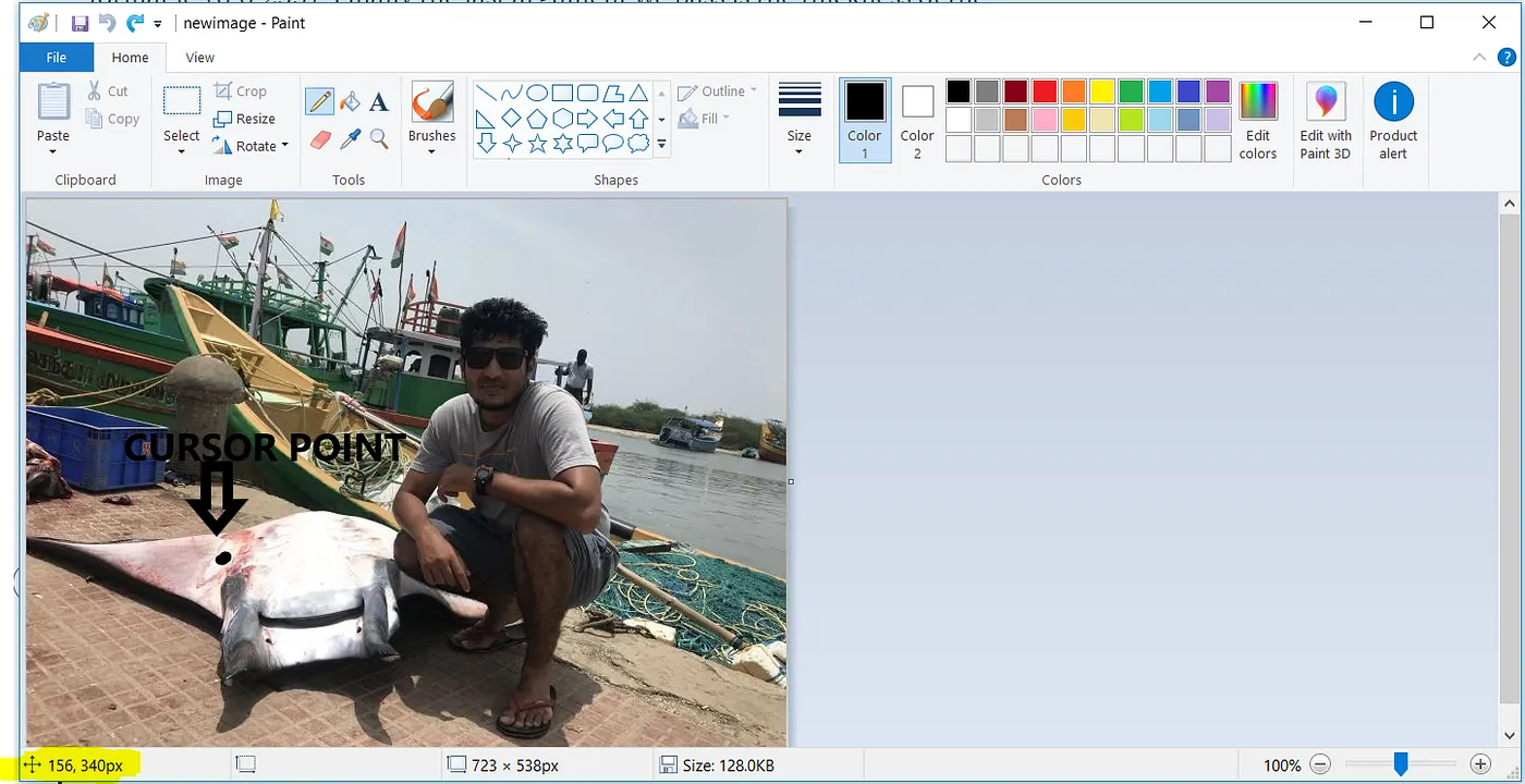
We will take the help of MS Paint for one more time. By placing the cursor over one of the co-ordinate (top left) or (bottom right) of the region to mask, the co-ordinates are shown in the highlighted portion of the MS Paint as shown in Fig 2.7.

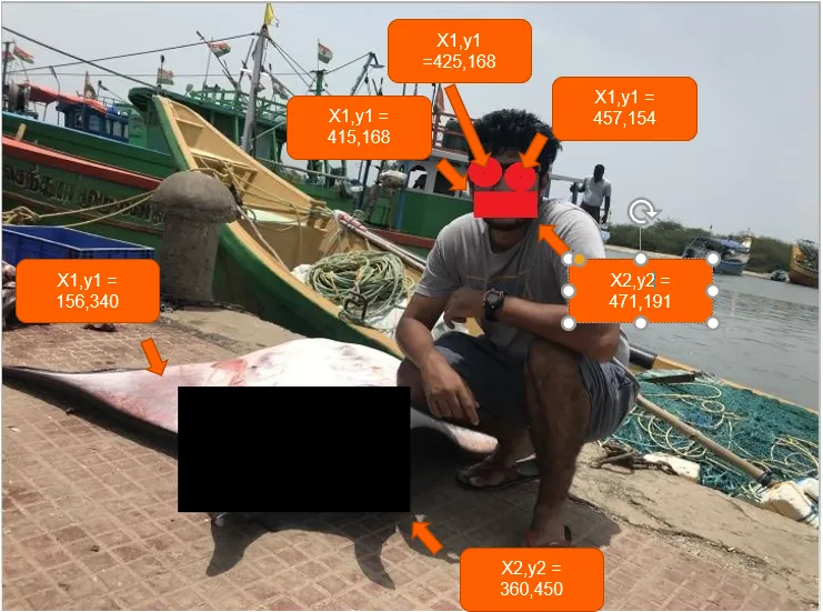
Similarly we will take all the co-ordinate (x1,y1) (x2,y2) for all the masking regions as shown in the Fig 2.8.

#Drawing using OpenCV to mask eyes,mouth and object near-by

import cv2
import argparse

apr = argparse.ArgumentParser()
apr.add_argument(“-i”, “ — image”, required=True, help=”Path to the image”)
args = vars(apr.parse_args())

image = cv2.imread(args[“image”])

cv2.rectangle(image, (415, 168), (471, 191), (0, 0, 255), -1)
cv2.circle(image, (425, 150), 15, (0, 0, 255), -1)
cv2.circle(image, (457, 154), 15, (0, 0, 255), -1)
cv2.rectangle(image, (156, 340), (360, 450), (0, 0, 0), -1)

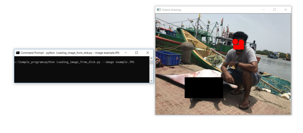
# show the output image
cv2.imshow(“Output drawing “, image)
cv2.waitKey(0)

Result: