Debugging Apache Spark Performance Using Explain Plan
When dealing with slow or stuck jobs, utilizing Spark's explain plan can help to better understand the internal processes and improve performance.
Join the DZone community and get the full member experience.
Join For FreeIn the world of data processing, Apache Spark has established itself as a powerful and versatile framework. However, as the volume and complexity of data continue to grow, ensuring optimal performance becomes paramount.
In this blog post, we will explore how the Explain Plan can be your secret weapon for debugging and optimizing Spark applications. We'll dive into the basics and provide clear examples in Spark Scala to help you understand how to leverage this valuable tool.
What Is the Explain Plan?
The Explain Plan is a comprehensive breakdown of the logical and physical execution steps that Spark follows to process your data. Think of it as a roadmap that guides you through the inner workings of your Spark job.
Two important components of Spark's Explain Plan are:
1. Logical Plan: The logical plan represents the high-level transformations and operations specified in your Spark application. It's an abstract description of what you want to do with your data.
2. Physical Plan: The physical plan, on the other hand, provides the nitty-gritty details of how Spark translates your logical plan into a set of concrete actions. It reveals how Spark optimizes your job for performance.
Explain API has a couple of other overloaded methods:
explain()- Prints the physical plan.explain(extended: Boolean)- Prints the plans (logical and physical).explain(mode: String)- Prints the plans (logical and physical) with a format specified by a given explain mode:simplePrint only a physical plan.extended: Print both logical and physical plans.codegen: Print a physical plan and generate codes if they are available.cost: Print a logical plan and statistics if they are available.formatted: Split explain output into two sections: a physical plan outline and node details.
Usage of Explain Plan
We can do this using the explain() method on a DataFrame or Dataset. Here's a simple example of using the Explain Plan:
import org.apache.spark.sql.SparkSession

// Create a SparkSession
val spark = SparkSession.builder()
  .appName("ExplainPlanExample")
  .getOrCreate()

// Create a dummy DataFrame for employees
val employeesData = Seq(
  (1, "Alice", "HR"),
  (2, "Bob", "Engineering"),
  (3, "Charlie", "Sales"),
  (4, "David", "Engineering")
)

val employeesDF = employeesData.toDF("employee_id", "employee_name", "department")

// Create another dummy DataFrame for salaries
val salariesData = Seq(
  (1, 50000),
  (2, 60000),
  (3, 55000),
  (4, 62000)
)

val salariesDF = salariesData.toDF("employee_id", "salary")

// Register DataFrames as SQL temporary tables
employeesDF.createOrReplaceTempView("employees")
salariesDF.createOrReplaceTempView("salaries")

// Use Spark SQL to calculate average salary per department
val avgSalaryDF = spark.sql("""
  SELECT department, AVG(salary) as avg_salary
  FROM employees e
  JOIN salaries s ON e.employee_id = s.employee_id
  GROUP BY department
""")


// call Explain Plan with extended mode to print both physical and logical plan
avgSalaryDF.explain(true)

// Stop the SparkSession
spark.stop()
In above example, we are creating a sample employeeData and salariesData DataFrames and performing a join and later aggregate to get the average salary by the department. Below is explain plan for the given dataframe.
scala> avgSalaryDF.explain(true)
== Parsed Logical Plan ==
'Aggregate ['department], ['department, 'AVG('salary) AS avg_salary#150]
+- 'Join Inner, ('e.employee_id = 's.employee_id)
   :- 'SubqueryAlias e
   :  +- 'UnresolvedRelation [employees], [], false
   +- 'SubqueryAlias s
      +- 'UnresolvedRelation [salaries], [], false

== Analyzed Logical Plan ==
department: string, avg_salary: double
Aggregate [department#135], [department#135, avg(salary#147) AS avg_salary#150]
+- Join Inner, (employee_id#133 = employee_id#146)
   :- SubqueryAlias e
   :  +- SubqueryAlias employees
   :     +- View (`employees`, [employee_id#133,employee_name#134,department#135])
   :        +- Project [_1#126 AS employee_id#133, _2#127 AS employee_name#134, _3#128 AS department#135]
   :           +- LocalRelation [_1#126, _2#127, _3#128]
   +- SubqueryAlias s
      +- SubqueryAlias salaries
         +- View (`salaries`, [employee_id#146,salary#147])
            +- Project [_1#141 AS employee_id#146, _2#142 AS salary#147]
               +- LocalRelation [_1#141, _2#142]

== Optimized Logical Plan ==
Aggregate [department#135], [department#135, avg(salary#147) AS avg_salary#150]
+- Project [department#135, salary#147]
   +- Join Inner, (employee_id#133 = employee_id#146)
      :- LocalRelation [employee_id#133, department#135]
      +- LocalRelation [employee_id#146, salary#147]

== Physical Plan ==
AdaptiveSparkPlan isFinalPlan=false
+- HashAggregate(keys=[department#135], functions=[avg(salary#147)], output=[department#135, avg_salary#150])
   +- Exchange hashpartitioning(department#135, 200), ENSURE_REQUIREMENTS, [plan_id=271]
      +- HashAggregate(keys=[department#135], functions=[partial_avg(salary#147)], output=[department#135, sum#162, count#163L])
         +- Project [department#135, salary#147]
            +- BroadcastHashJoin [employee_id#133], [employee_id#146], Inner, BuildRight, false
               :- LocalTableScan [employee_id#133, department#135]
               +- BroadcastExchange HashedRelationBroadcastMode(List(cast(input[0, int, false] as bigint)),false), [plan_id=266]
                  +- LocalTableScan [employee_id#146, salary#147]


scala>
As you can see above, with extended flag set to true, we have Parsed Logical Plan, Analyzed Logical Plan, Optimized Logical Plan, and Physical Plan.
Before trying to understand plans, we need to read all plans bottom up. So we will see any dataframe creation or reads at bottom.
We will understand each one of these:
Parsed Logical Plan
This is the initial stage where Spark parses the SQL or DataFrame operations provided by the user and creates a parsed representation of the query. When using spark SQL query, any syntax errors are caught here. If we observe here, column names are not yet resolved.
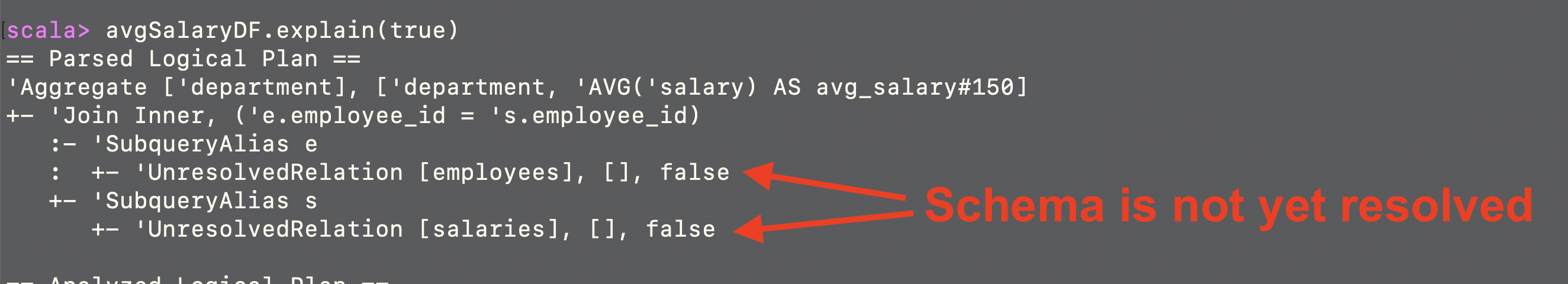 In the above parsed logical plan, we can see UnresolvedRelation. It means that schema is not yet resolved. The parsed logical plan outlines the logical structure of the query, including the aggregation and join operations. It also defines the aliases and identifies the sources of the
 employees and salaries DataFrames. The unresolved relations will be resolved to their actual data sources during query execution.
Analyzed Logical Plan
After parsing, Spark goes through a process called semantic analysis or resolution. In this stage, Spark checks the query against the catalog of available tables and columns, resolves column names, verifies data types, and ensures that the query is semantically correct. The result is an analyzed logical plan that incorporates metadata and information about the tables and columns involved.
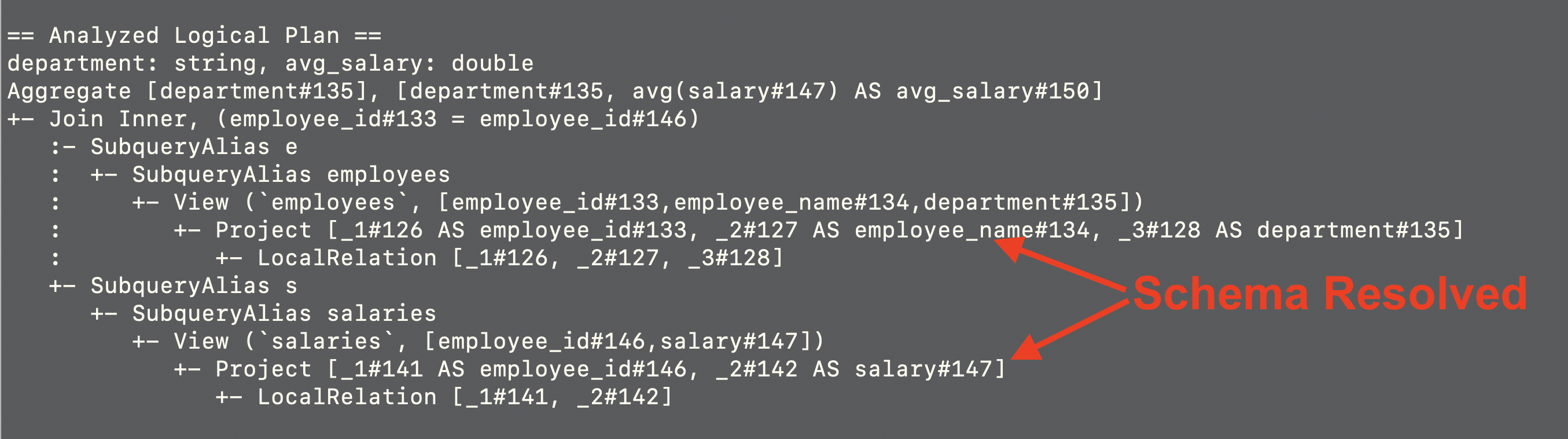 This plan represents the initial logical structure of your query after parsing and semantic analysis. It shows the result schema with two columns,
 department and avg_salary. The plan consists of two subqueries, e, and s, which correspond to the employees and salaries DataFrames. The inner join operation is applied between these subqueries using employee_id as the join key. The plan also includes aliases (e and s) and projection operations to select specific columns.
Optimized Logical Plan
Once the query is analyzed and Spark has a clear understanding of the data and schema, it proceeds to optimize the query. During optimization, Spark applies various logical optimizations to the query plan to improve performance. This may involve techniques like predicate pushdown, constant folding, and rule-based transformations. The optimized logical plan represents a more efficient version of the query in terms of data retrieval and processing.
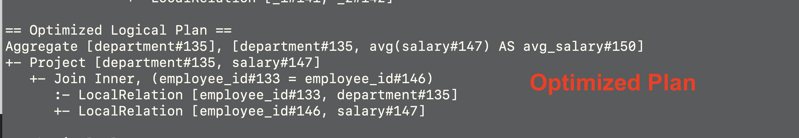 The optimization phase simplifies the plan for better performance. In this case, the plan is simplified to remove subqueries and unnecessary projection operations. It directly joins the two local relations (
employees and salaries) using the employee_id join key and then applies the aggregation for calculating the average salary per department.
Physical Plan
The physical plan, also known as the execution plan, is the final stage of query optimization. At this point, Spark generates a plan for how the query should be physically executed on the cluster. It considers factors such as data partitioning, data shuffling, and task distribution across nodes. The physical plan is the blueprint for the actual execution of the query, and it takes into account the available resources and parallelism to execute the query efficiently.
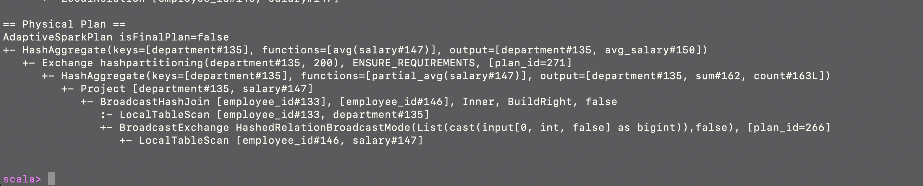 The physical plan outlines the actual execution steps taken by Spark to perform the query. It involves aggregation, joins, and data scans, along with optimization techniques like broadcast join for efficiency. This plan reflects the execution strategy that Spark will follow to compute the query result. Now, lets go over each line to understand much deeper (going from bottom to top).
- LocalTableScan: These are scans of local tables. In this case, they represent the tables or DataFrames
employee_id#133,department#135,employee_id#146, andsalary#147. These scans retrieve data from the local partitions. - BroadcastExchange: This operation broadcasts the smaller DataFrame (
employee_id#146andsalary#147) to all worker nodes for the broadcast join. It specifies the broadcast mode asHashedRelationBroadcastModeand indicates that the input data should be broadcasted. - BroadcastHashJoin: This is a join operation between two data sources (
employee_id#133andemployee_id#146) using aninner join. It builds the right side of the join as it is marked as "BuildRight". This operation performs a broadcast join, which means it broadcasts the smaller DataFrame (right side) to all nodes where the larger DataFrame (left side) resides. This is done for optimization purposes when one DataFrame is significantly smaller than the other. - Project: This operation selects the
departmentandsalarycolumns from the data. - HashAggregate (partial_avg): This is a partial aggregation operation that computes the average salary for each department. It includes additional columns,
sum#162andcount#163L, which represent the sum of salaries and the count of records, respectively. - Exchange hashpartitioning: This operation performs a hash partitioning of the data based on the
department#135column. It aims to distribute the data evenly among 200 partitions. TheENSURE_REQUIREMENTSattribute suggests that this operation ensures the requirements of the subsequent operations. - HashAggregate: This is an aggregation operation that calculates the average salary (
avg(salary#147)) for each unique value in thedepartmentcolumn. The output includes two columns:department#135andavg_salary#150. - AdaptiveSparkPlan: This represents the top-level execution plan for the Spark query. The attribute
isFinalPlan=falsesuggests that this plan is not yet finalized, indicating that Spark may adapt the plan during execution based on runtime statistics.
Conclusion
Understanding the execution plan generated by Spark SQL is immensely valuable for developers in several ways:
- Query Optimization: By examining the physical plan, developers can gain insights into how Spark optimizes their SQL queries. It helps them see if the query is efficiently using available resources, partitions, and joins.
- Performance Tuning: Developers can identify potential performance bottlenecks in the plan. For instance, if they notice unnecessary shuffling or data redistribution, they can revise their query or adjust Spark configurations to improve performance.
- Debugging: When queries do not produce the expected results or errors occur, the physical plan can provide clues about where issues might be. Developers can pinpoint problematic stages or transformations in the plan.
- Efficient Joins: Understanding join strategies like broadcast joins helps developers make informed decisions about which tables to broadcast. This can significantly reduce the shuffle and improve query performance.
Opinions expressed by DZone contributors are their own.
Comments