How Much Signal Differential Privacy Takes From Your Dashboards, in Events

Somebody ships a differential privacy layer in front of the event store and leaves the dashboards sitting on top of it. The queries still return, the totals still look like totals, and the ticket gets closed. Nobody on the team computed the floor.

Every private aggregate carries noise, and the noise is unlabeled. It sits in the same cell somebody reads on Monday morning before deciding whether a segment moved, and to the eye it looks like a small real change. In the ad-account work I do, the move to aggregate and private reporting comes from regulation rather than from architecture, so the debate never really happens, and the pattern is always the same: epsilon gets negotiated in a meeting, and the arithmetic that would turn it into a detection limit never makes it into any document.

That conversion is four lines. The rest of this runs them against schema choices teams actually ship.

Name the Unit Before Anything Else

Differential privacy protects a unit, and you have to say which one. Everything below assumes user-level privacy: add or remove one user together with all of their events.

That choice causes most of the confusion that shows up later. The textbook line, a histogram has sensitivity 1 no matter how many buckets it has, is an event-level statement. One row in, one row out. Under user-level privacy, a single user can drop forty events into one cell, and forty is your sensitivity.

So one quantity runs through every formula below: the largest total contribution one user can make to one release, in the units of the metric. Events, for counting queries. It is a cap you write into the job. You do not get it from a MAX() over yesterday's users. Wilson and colleagues (2020) built exactly this into a production SQL engine, because a query with no bound has no calibrated noise to add.

With that in hand, the Laplace mechanism is a one-liner: noise of scale b = bound / epsilon (Dwork, McSherry, Nissim and Smith, 2006), and a single noisy count with standard deviation b * sqrt(2).

The Number That Belongs in a Schema Review

The cell people argue about is almost always a difference, this week minus last week or treatment minus holdout or one region minus the next.

The difference of two independent Laplace variables is not Gaussian, and the shortcut is off by enough to matter. For Z = Lap(b) - Lap(b) the exact two-sided tail is exp(-t/b) * (1 + t/(2b)). Set it to 0.05, and the critical value is 4.11b. The normal approximation gives 1.96 * 2b = 3.92b, an interval that in fact covers 94.1%. Reviewers do not catch the missing 5.9% of coverage, because the chart still has two lines on it.

Schema review needs a different number anyway. Significance is the question you ask once a movement is already on the screen. Before the pipeline ships, what you need is the size of movement it can be expected to catch at all. At 80% power that comes out at 5.58b, taken from the exact law and then checked by simulation. Treating the Gaussian 3.92b as if it were the detection floor is the substitution that flatters the pipeline.

import math, random

def tail(u):                       # P(|Lap(b) - Lap(b)| > u*b)
    return math.exp(-u) * (1 + u / 2)

def critical_value(alpha=0.05, lo=0.0, hi=60.0):
    for _ in range(200):
        mid = (lo + hi) / 2
        lo, hi = (mid, hi) if tail(mid) > alpha else (lo, mid)
    return (lo + hi) / 2           # in units of b

def schema_cost(epsilon, per_user_bound, releases):
    """What one release costs you in events, given a user-level bound."""
    b = per_user_bound * releases / epsilon     # basic sequential composition
    crit = critical_value()
    return b, b * math.sqrt(2), crit * b, 5.578 * b

for label, bound, releases in [
        ("one event per user, published once", 1, 1),
        ("bound 24 events per user, published once", 24, 1),
        ("bound 24, republished nightly for a month", 24, 30),
        ("bound 5, republished nightly for a month", 5, 30)]:
    b, sd, crit, mde = schema_cost(1.0, bound, releases)
    print(f"{label:44s} b={b:7.1f} sd={sd:8.1f} "
          f"significant above={crit:8.1f} 80% power needs={mde:9.1f}")

At epsilon = 1.0:

one event per user, published once           b=    1.0 sd=     1.4 significant above=     4.1 80% power needs=      5.6
bound 24 events per user, published once     b=   24.0 sd=    33.9 significant above=    98.7 80% power needs=    133.9
bound 24, republished nightly for a month    b=  720.0 sd=  1018.2 significant above=  2961.4 80% power needs=   4016.2
bound 5, republished nightly for a month     b=  150.0 sd=   212.1 significant above=   617.0 80% power needs=    836.7

All four rows spend the same epsilon. On the first row, 80% power is six events. On the third, it is four thousand. The only things that moved are the per-user bound and the nightly refresh.

The bound and the refresh get treated as one knob, and they do not move the same quantity.

The bound is what you pay for, and coarsening does not lower it. Roll hourly buckets up into six-hour blocks, and one user's total contribution across the release is what it was, so b sits where it was. Coarsening still helps, only through the denominator: more events per cell means the same absolute noise is a smaller share of it.

Releases accumulate. A nightly job over a rolling window is thirty releases in a month, and under basic composition each one gets epsilon / 30. Teams count dashboards and then spend the budget on refresh cadence, including tiles that never get opened.

Flat Noise, Very Unflat Keys

Noise is added at one scale for every cell. Real event mass is not, and the gap is where a private report stays readable on the top row and falls apart below it.

Two measurements from a corpus I work with, roughly 24 million rows of ad-account data. In one product niche, a single three-word search query takes between 6.5% and 41.6% of an account's total spend, median near 17.7% across six competitors. Across seven product categories in the same corpus, the share of spend sitting in one country runs from 10.8% to 81.1%.

Those two figures are spend shares, not event counts, and they describe spread across accounts rather than neighboring cells inside one report. I am not using them as a stand-in for cell mass. I use them for the shape: in data of this kind, one key routinely carries a double-digit percentage of everything, and the rest of the distribution drops off fast. What the simulation below reproduces is that shape; the corpus itself never enters the code.

def laplace(rnd, b):
    u = rnd.random() - 0.5
    return -b * math.copysign(1.0, u) * math.log(1.0 - 2.0 * abs(u))

def skew(total, keys, b, tol=0.10, reps=300, seed=7):
    rnd = random.Random(seed)
    w = [1.0 / i for i in range(1, keys + 1)]
    w = [x / sum(w) for x in w]                  # heavy head, long tail
    truth = [total * x for x in w]
    over_keys, over_mass = 0, 0.0
    for _ in range(reps):
        rel = [abs(laplace(rnd, b)) / t for t in truth]
        idx = [i for i, r in enumerate(rel) if r > tol]
        over_keys += len(idx)
        over_mass += sum(w[i] for i in idx)
    return 100 * over_keys / (reps * keys), 100 * over_mass / reps

for tag, b in [("bound 24, 30 releases (b=720)", 720.0),
               ("bound 5, 30 releases (b=150)", 150.0),
               ("bound 24, one release (b=24)", 24.0)]:
    pct_keys, pct_mass = skew(100_000, 720, b)
    print(f"{tag:32s} keys over 10% error={pct_keys:5.1f}%  events in them={pct_mass:5.1f}%")

bound 24, 30 releases (b=720)    keys over 10% error= 98.4%  events in them= 74.9%
bound 5, 30 releases (b=150) keys over 10% error= 93.9% events in them= 53.2%
bound 24, one release (b=24)     keys over 10% error= 76.0%  events in them= 28.2%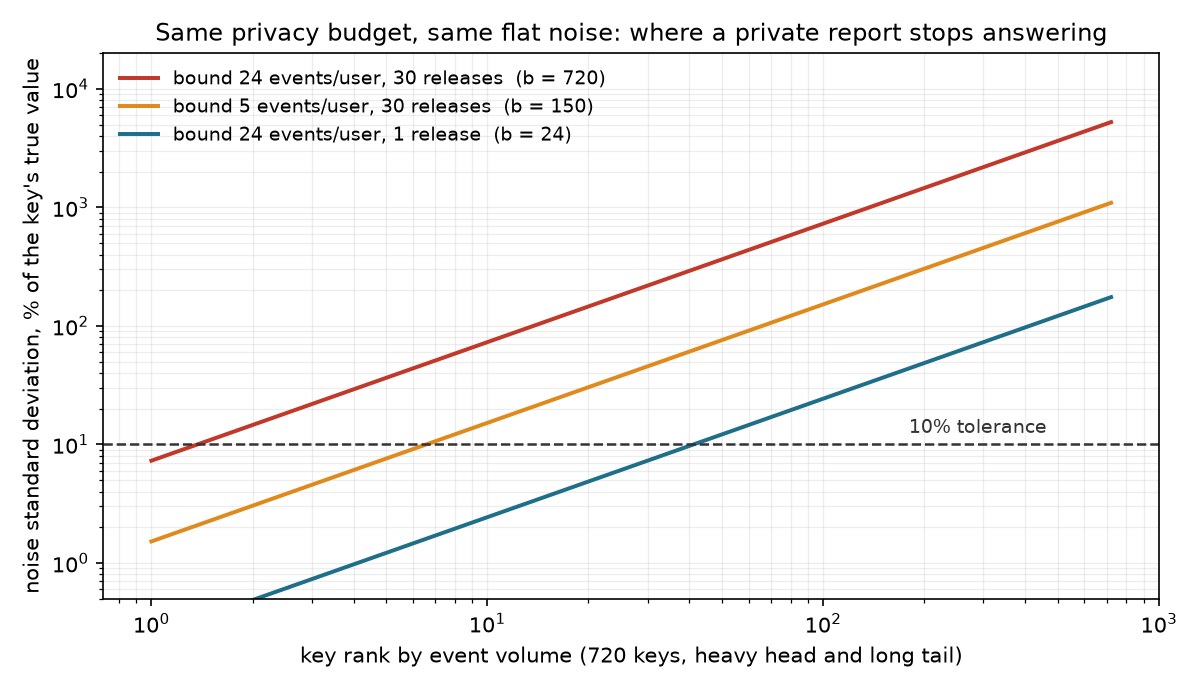

The top key holds 14% of all events and carries about 7% relative noise, so the headline stays healthy. The tenth-largest key is already past 50%. Rank 100 sits at 729%. Half the events live in the top twenty keys. Volume can look fine while almost every key in the same release is already unusable, and the chart does not flag which cells are which.

Five Lines for the Schema Review

• Write the decision threshold next to the query, in events. If 5.58 * b is bigger than the difference that would change what you do, the query cannot answer it at this budget, and no amount of chart work fixes that.
• The per-user bound is a decision you make once and then live with. Tightening it from 24 to 5 brought that floor down by a factor of almost five in the table above. It also censors your heaviest users, so part of the variance you win comes back as bias. Measure how much you clip and report it beside the estimate.
• Resolution is bought by raising cell mass: coarser keys, longer windows, fewer dimensions per release. b stays where it was; what improves is the noise-to-mass ratio.
• Budget accrues per release, not per dashboard. Refreshes, backfills, and one-off reruns over the same users all spend it.
• A non-private control aggregate is for internal audit and stays there. Published next to the private number, the difference between the two is the noise, handed back in clear.

The architecture choice sits underneath all five. Local differential privacy of the RAPPOR kind (Erlingsson, Pihur and Korolova, 2014) moves the noise onto the client, and for the same epsilon the floor lands much higher, with no amount of schema work bringing it back down. Shuffling designs such as Prochlo (Bittau and colleagues, 2017) change the trust model, and the arithmetic changes with it. Every number above assumes the central model, so a team that has not settled its trust boundaries cannot quote a floor to anyone.

Where This Stops

This is about measurement precision, not delivery. An aggregate can tell you an effect exists; it cannot restore per-user selection to a system that lost it.

Small cells stay lost no matter what you set. The working rule is relative: if a cell's true count is not several times b * sqrt(2), fold it into a larger bucket instead of publishing a number you cannot defend. Which cells qualify depends on your bound and your release count, so the threshold is local to the pipeline.

One thing I have not measured: how much of a causal estimate survives an end-to-end private stack, where on-device selection feeds an aggregated reporting API. I would like that number from anyone running it in production, specifically how wide the confidence interval on a lift estimate ends up at the far side. I have not seen it characterized in public, and it determines whether private measurement is good for decisions or only for reporting.

It is an afternoon of work, and it has to happen before go-live. After that, nobody in the building can say which part of a movement was the noise.

References

1. Dwork, C., McSherry, F., Nissim, K., Smith, A. (2006). Calibrating Noise to Sensitivity in Private Data Analysis. Theory of Cryptography, LNCS, 265-284. https://doi.org/10.1007/11681878_14
2. Wilson, R. J., Zhang, C. Y., Lam, W., Desfontaines, D., Simmons-Marengo, D., Gipson, B. (2020). Differentially Private SQL with Bounded User Contribution. Proceedings on Privacy Enhancing Technologies, 2020(2), 230-250. https://doi.org/10.2478/popets-2020-0025
3. Erlingsson, U., Pihur, V., Korolova, A. (2014). RAPPOR: Randomized Aggregatable Privacy-Preserving Ordinal Response. ACM CCS 2014, 1054-1067. https://doi.org/10.1145/2660267.2660348
4. Bittau, A., Erlingsson, U., Maniatis, P., Mironov, I., Raghunathan, A., Lie, D., Rudominer, M., Kode, U., Tinnes, J., Seefeld, B. (2017). Prochlo: Strong Privacy for Analytics in the Crowd. SOSP 2017, 441-459. https://doi.org/10.1145/3132747.3132769