Google Colab: Create Predictive Models in No Time
In this article, we will see how we can use this amazing cloud-based platform and use a Random Forest model to predict customer churn in less than 200 lines of code.
Join the DZone community and get the full member experience.
Join For FreeTo democratize data analytics and do all the data munging related heavy lifting, let's explore Google's Colaboratory, which is a Jupyter notebook environment that requires no setup and runs entirely on the cloud. Google's Colaboratory is a perfect solution for today's data analysts and engineers. In this article, we will see how we can use this amazing cloud-based platform and use a Random Forest model to predict customer churn in less than 200 lines of code.
Before we start, I would like to point out some great capabilities that Google Colab environment has in store for its users.
- No more dependency on the dependencies: You talk about any programming language, Google Colab has got all the required packages and dependencies already installed. This saves a lot of time and effort, given the fact that there are thousands of such dependencies available to make data analytics a breeze.
- CPU to GPU to TPU: This is one of the most exciting and amazing features of Google Colab. As I stated above, Google Colab will do all the data processing and crunching-related heavy lifting on its own without worrying about the capacity of the user's physical machine. Considering the fact that Google Colab is a cloud-based platform. allowing its users to experience the true power of the cloud-based application, itwill be worth stating the key differences in between CPU, GPU, and TPU
- CPU: Going by its text book definition, a Central Processing Unit is the electronic circuitry which is considered the brain of the computer and is used to perform the basic arithmetic, logical, control, and input/output operations specified by the instructions of a computer application.
- GPU: A Graphics Processing Unit is a high-end circuitry that is designed to render 2D and 3D graphics together with the CPU. However, nowadays GPUs are being used to do all the heavy data crunching to accelerate the computational workloads while developing any model.
- TPU: A Tensor Processing Unit is custom made circuitry developed specifically to execute machine learning and Tensor Flow, Google's open source machine learning framework.
Now that we have some basic understanding of the Google Colaboratory environment and its key features, we can get started with a very basic routine that we will deploy using the Google Colaboratory environment. To demonstrate the ease of use we will be using our all-time favorite data science language, Python.
Before we get started, I just want to call out that this is not a tutorial article on the Python language. This article is just to demonstrate the ease of use and simplicity of the Google Colab environment.
Let's get started!
Once you have fired up your Google Colab environment, its time to call all the required libraries for this modeling routine.
import pandas as pd
from sklearn.model_selection import train_test_split
from sklearn.ensemble import RandomForestClassifier
from sklearn.metrics import confusion_matrix
from sklearn.metrics import roc_curve
import matplotlib
import matplotlib.pyplot as plt
from IPython.display import display, HTML
Once all the dependencies have been called, it is time to use them. Using the Pandas read.csv command we will read the customer data file. Using the below code we should be able to see the 5 rows of our customer data set.
df = pd.read_csv("Customer Churn Data.csv")
display(df.head(5))
Though the data that I am using is a made-up or dummy data and all the values are in binaries, I will still go ahead and use the Pandas shape data frame function to look at the rows and column counts.
print("Number of rows: ", df.shape[0])
counts = df.describe().iloc[0]
display(
pd.DataFrame(
counts.tolist(),
columns=["Count of values"],
index=counts.index.values
).transpose()
)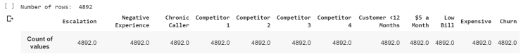 Now let's split the data into training and test:
df_train, df_test = train_test_split(df, test_size=0.25)Fire up the random forest model by calling it!
clf = RandomForestClassifier(n_estimators=30)
clf.fit(df_train[features], df_train["Churn"])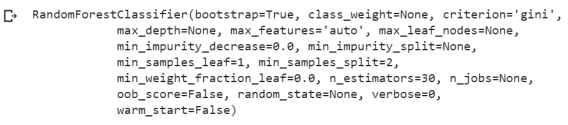 Make some predictions:
predictions = clf.predict(df_test[features])
probs = clf.predict_proba(df_test[features])
display(predictions)
Evaluate the model:
score = clf.score(df_test[features], df_test["Churn"])
print("Accuracy: ", score)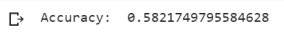 Create a confusion matrix and ROC:
get_ipython().magic('matplotlib inline')
confusion_matrix = pd.DataFrame(
confusion_matrix(df_test["Churn"], predictions),
columns=["Predicted False", "Predicted True"],
index=["Actual False", "Actual True"]
)
display(confusion_matrix)

# Calculate the fpr and tpr for all thresholds of the classification
fpr, tpr, threshold = roc_curve(df_test["Churn"], probs[:,1])
plt.title('Receiver Operating Characteristic')
plt.plot(fpr, tpr, 'b')
plt.plot([0, 1], [0, 1],'r--')
plt.xlim([0, 1])
plt.ylim([0, 1])
plt.ylabel('True Positive Rate')
plt.xlabel('False Positive Rate')
plt.show()
Now you can check the results by deploying the model that you have created on the test data.
df_test["prob_true"] = probs[:, 1]
df_risky = df_test[df_test["prob_true"] > 0.9]
display(df_risky.head(5)[["prob_true"]])
When I create the very first version of any model, I go full throttle. This means that I use all the variables. If I see that my model is too accurate or totally useless from the perspective of its accuracy score than I deploy the feature selection method. Some may agree with this approach and some may not, but it is more of personal preference.
fig = plt.figure(figsize=(20, 18))
ax = fig.add_subplot(111)

df_f = pd.DataFrame(clf.feature_importances_, columns=["importance"])
df_f["labels"] = features
df_f.sort_values("importance", inplace=True, ascending=False)
display(df_f.head(5))

index = np.arange(len(clf.feature_importances_))
bar_width = 0.5
rects = plt.barh(index , df_f["importance"], bar_width, alpha=0.4, color='b', label='Main')
plt.yticks(index, df_f["labels"])
plt.show()
So we can clearly see that in less than 200 lines of code, I have been able to create a pretty decent Random Forest model using dummy data with an accuracy which is better than a flip of a coin.
The original model can be accessed on my GitHub site - Access it here!
Published at DZone with permission of Sunil Kappal. See the original article here.
Opinions expressed by DZone contributors are their own.
Comments