Apache Cassandra Essentials

Apache Cassandra is a performance-oriented, extremely scalable, fault-tolerant (i.e., no single point of failure), distributed non-relational database solution. Teams typically consider Cassandra, along with Google Bigtable, Amazon DynamoDB, and ScyllaDB, to handle the types of database management needs that traditional RDBMS vendors cannot support.

Cassandra is in use by many of the world's largest engineering teams: Apple (75,000+ nodes), Spotify (3,000+ nodes), Bloomberg, Uber, Verizon, Adobe, Netflix, and more companies that have large datasets and dedicated Cassandra specialists (often Cassandra committers) on staff.

The table below details several primary differences between RDBMSs and Cassandra:

Cassandra has a tabular schema comprising keyspaces, tables, partitions, rows, and columns:

Schema

The keyspace is akin to a database or schema in an RDBMS, contains a set of tables, and is used for replication. A keyspace and table is the unit for Cassandra's access control mechanism. When enabled, users must authenticate to access and manipulate data in a schema or table.

Table

A table, previously known as a column family, is a map of rows. Similar to an RDBMS, a table is defined by a primary key, which consists of a partition key and clustering columns. The partition key defines data locality in the cluster, and the data with the same partition key will be stored together on a single node. The clustering columns define how the data will be ordered on the disk within a partition. The client application provides rows that conform to the schema. Each row has the same fixed subset of columns.

As values for these properties, Cassandra provides the following Cassandra Query Language (CQL) data types for columns (see the Apache Cassandra documentation):

Rows 

Cassandra supports tables defined with composite primary keys. The first part of the primary key is a partition key. Remaining columns are clustering columns and define the order of the data on the disk. For example, let's say there is a table called users_by_location with the following primary key:

((country, town), birth_year, user_id)

In that case, the (country, town) pair is a partition key (a composite one). All users with the same (country, town) values will be stored together on a single node and replicated together based on the replication factor. The rows within the partition will be ordered by birth_year and then by user_id. The user_id column provides uniqueness for the primary key.

If the partition key is not separated by parentheses, the first column in the primary key is considered a partition key. For example, if the primary key is defined by (country, town, birth_year, user_id), country would be the partition key and town would be a clustering column.

Columns

A column is a triplet: key, value, and timestamp. The validation and comparator on the column family define how Cassandra sorts and stores the bytes in column keys. The timestamp portion of the column is used to sequence mutations; it is defined and specified by the client. Newer versions of Cassandra drivers provide this functionality out of the box. Client application servers should have synchronized clocks. 

Columns may optionally have a time to live (TTL), after which Cassandra asynchronously deletes them. Note that TTLs are defined per cell, so each cell in the row has an independent TTL and is handled by Cassandra independently.

How Data Is Stored on the Disk

Using the sstabledump tool, you can inspect how the data is stored on the disk. This is very important if you want to develop intuition about data modeling, reads, and writes in Cassandra.

For example, given the table defined by:

CREATE TABLE IF NOT EXISTS symbol_history (
  symbol         text,
  year           int,
  month          int,
  day            int,
  volume         bigint,
  close          double,
  open           double,
  low            double,
  high           double,
  idx            text static,
  PRIMARY KEY ((symbol, year), month, day)
) with CLUSTERING ORDER BY (month desc, day desc);

The data (when deserialized into JSON using the sstabledump tool) is stored on the disk in this form:

[
  {
    "partition" : {
      "key" : [ "CORP", "2016" ],
      "position" : 0
    },
    "rows" : [
      {
        "type" : "static_block",
        "position" : 48,
        "cells" : [
          { "name" : "idx", "value" : "NASDAQ", 
"tstamp" : 1457484225583260, "ttl" : 604800, "expires_
at" : 1458089025, "expired" : false }
        ]
      },
      {
        "type" : "row",
        "position" : 48,
        "clustering" : [ "1", "5" ],
        "deletion_info" : { "deletion_time" : 
1457484273784615, "tstamp" : 1457484273 }
      },
      {
        "type" : "row",
        "position" : 66,
        "clustering" : [ "1", "4" ],
        "liveness_info" : { "tstamp" : 
1457484225586933, "ttl" : 604800, "expires_at" : 
1458089025, "expired" : false },
        "cells" : [
          { "name" : "close", "value" : "8.54" },
          { "name" : "high", "value" : "8.65" },
          { "name" : "low", "value" : "8.2" },
          { "name" : "open", "value" : "8.2" },
          { "name" : "volume", "value" : "1054342" }
        ]
      },
      {
        "type" : "row",
        "position" : 131,
        "clustering" : [ "1", "1" ],
        "liveness_info" : { "tstamp" : 
1457484225583260, "ttl" : 604800, "expires_at" : 
1458089025, "expired" : false },
        "cells" : [
          { "name" : "close", "value" : "8.2" },
          { "name" : "high", "deletion_time" : 
1457484267, "tstamp" : 1457484267368678 },
          { "name" : "low", "value" : "8.02" },
          { "name" : "open", "value" : "9.33" },
          { "name" : "volume", "value" : "1055334" }
        ]
      }
    ]
  },
  {
    "partition" : {
      "key" : [ "CORP", "2015" ],
      "position" : 194
    },
    "rows" : [
      {
        "type" : "static_block",
        "position" : 239,
        "cells" : [
          { "name" : "idx", "value" : "NYSE", "tstamp"
 : 1457484225578370, "ttl" : 604800, "expires_at" : 
1458089025, "expired" : false }
        ]
      },
      {
        "type" : "row",
        "position" : 239,
        "clustering" : [ "12", "31" ],
        "liveness_info" : { "tstamp" : 
1457484225578370, "ttl" : 604800, "expires_at" : 
1458089025, "expired" : false },
        "cells" : [
          { "name" : "close", "value" : "9.33" },
          { "name" : "high", "value" : "9.57" },
          { "name" : "low", "value" : "9.21" },
          { "name" : "open", "value" : "9.55" },
          { "name" : "volume", "value" : "1054342" }
        ]
      }
    ]
  }
]

Cassandra was designed to support high write throughput and be horizontally scalable without sacrificing read efficiency.

Infrastructure Selection

Cassandra's architecture is optimized for deployment on commodity hardware, enabling organizations to build cost-effective, expansive clusters using numerous small, inexpensive servers. This approach allows for horizontal scaling through many low-cost nodes. However, be aware that this can introduce significant operational challenges at scale. Managing and maintaining large clusters requires substantial administrative overhead and complex synchronization of node health, data replication, and performance monitoring across the distributed infrastructure. Lower-end hardware is also less efficient in computing and I/O, which translates to elevated operation latencies.

Ring Architecture

A cluster is a collection of nodes that Cassandra uses to store the data. The nodes are logically distributed like a ring. A minimum cluster typically consists of at least three nodes (minimum), but it can also have hundreds of nodes in it. Data is automatically replicated across the cluster, depending on the replication factor.

When deploying to the cloud or in a data center designed for high availability, each physical location (a zone in cloud terms) can be recognized by Cassandra as an isolated unit, called a rack, which allows for data placement alongside each rack. This means that if a zone or rack loss occurs, there are still two fully functioning copies of the data on the cluster in order to continue to fulfill highly available operations.

A Cassandra cluster is often referred to as a ring architecture, based on a hash ring — the way the cluster knows how to distribute data across the different nodes. A cluster can change size over time, adding more nodes (to expand storage and processing power) or removing nodes (either through purposeful decommissioning or system failure). When a topology change occurs, the cluster is designed to reconfigure itself and rebalance the data held within it automatically.

Within the cluster, all inter-node communication is peer to peer, so there is no single point of failure. For communication outside the cluster (e.g., read, write), a Cassandra client will communicate with a single server node, called the coordinator. The selection of the coordinator is made with each client connection request to prevent bottlenecking requests through a single node. This is further explained later on in this lesson.

A partition key is one or more columns that are responsible for data distribution across the nodes, and it determines in which nodes to store a given row. As we will see later on, typically, data is replicated, and copies are stored on multiple nodes. This means that even if one node goes down, the data will still be available. It ensures reliability and fault tolerance.

Replication

Cassandra provides continuous high availability and fault tolerance through data replication. The replication uses the ring to determine nodes used for replication. Replication is configured on the keyspace level. Each keyspace has an independent replication factor, n. When writing information, the data is written to the target node as determined by the partitioner and n-1 subsequent nodes along the ring.

There are two replication strategies: SimpleStrategy and NetworkTopologyStrategy.

SimpleStrategy

SimpleStrategy is the default strategy and blindly writes the data to subsequent nodes along the ring. This strategy is not recommended for a production environment. In the previous example with a replication factor of 2, this would result in the following storage allocation:

REPLICA 1 is determined by the partitioner, and REPLICA 2 is found by traversing the ring.

NetworkTopologyStrategy

NetworkTopologyStrategy is useful when deploying to multiple data centers, and it ensures that data is replicated across data centers. Effectively, NetworkTopologyStrategy executes the SimpleStrategy independently for each data center, spreading replicas across distant racks. Cassandra writes a copy in each data center as determined by the partitioner.

Data is written simultaneously along the ring to subsequent nodes within that data center, with preference for nodes in different racks to offer resilience to hardware failure. All nodes are peers, and data files can be loaded through any node in the cluster, eliminating the single point of failure inherent in a primary-coordinator architecture and making Cassandra fully fault-tolerant and highly available.

Figure 1: Ring and deployment topology

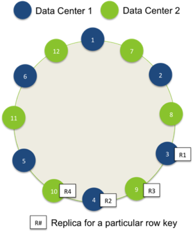
With blue nodes deployed to one data center (DC1), green nodes deployed to another data center (DC2), and a replication factor of 2 per each data center, one row will be replicated twice in DC1 (R1, R2) and twice in DC2 (R3, R4).

Note: Cassandra attempts to write data simultaneously to all target nodes, then waits for confirmation from the relevant number of nodes needed to satisfy the specified consistency level.

Consistency Levels

One of the unique characteristics of Cassandra that sets it apart from other databases is its approach to consistency. Clients can specify the consistency level on both read and write operations, trading off between high availability, consistency, and performance.

Write consistency levels:

Read consistency levels:

Network Topology

As input into the replication strategy and to efficiently route communication, Cassandra uses a snitch to determine the data center and rack of the nodes in the cluster. A snitch is a component that detects and informs Cassandra about the network topology of the deployment. The snitch dictates what is used in the strategy options to identify replication groups when configuring replication for a keyspace.

The following table shows the snitches provided by Cassandra and what you should use in your keyspace configuration for each snitch:

SimpleSnitch

SimpleSnitch provides Cassandra no information regarding racks or data centers. It is the default setting and is useful for simple deployments where all servers are collocated. It is not recommended for a production environment as it does not provide failure tolerance.

PropertyFileSnitch

PropertyFileSnitch allows users to be explicit about their network topology. The user specifies the topology in a properties file, cassandra-topology.properties. The file specifies what nodes belong to which racks and data centers. Below is an example property file for our sample cluster:

# DC1
192.168.0.1=DC1:RAC1
192.168.0.2=DC1:RAC1
192.168.0.3=DC1:RAC2

# DC2
192.168.1.4=DC2:RAC3
192.168.1.5=DC2:RAC3
192.168.1.6=DC2:RAC4

# Default for nodes
default=DC3:RAC5

GossipingPropertyFileSnitch

GossipingPropertyFileSnitch is recommended for production. It uses rack and data center information for the local node defined in the cassandra-rackdc.properties file and propagates this information to other nodes via gossip. Unlike PropertyFileSnitch, which contains topology for the entire cluster on every node, GossipingPropertyFileSnitch contains DC and rack information only for the local node. Each node describes and gossips its location to other nodes.

Example contents of the cassandra-rackdc.properties file:

dc=DC1
rack=RACK1

RackInferringSnitch

RackInferringSnitch

RackInferringSnitch infers network topology by convention. From the IPv4 address (e.g., 9.100.47.75), the snitch uses the following convention to identify the data center and rack:

EC2Snitch

EC2Snitch is useful for deployments to Amazon's EC2. It uses Amazon's API to examine the regions to which nodes are deployed. It then treats each region as a separate data center.

EC2MultiRegionSnitch

Use EC2MultiRegionSnitch for deployments on Amazon EC2, where the cluster spans multiple regions. This snitch treats data centers and availability zones as racks within a data center, and uses public IPs as broadcast_address to allow cross-region connectivity. Cassandra nodes in one EC2 region can bind to nodes in another region, thus enabling multi-data center support.

Note: Pay attention to which snitch and file you are using to define the topology. Some snitches use the cassandra-topology.properties file and other, newer snitches use cassandra-rackdc.properties.

GoogleCloudSnitch and AzureSnitch

GoogleCloudSnitch and AzureSnitch are useful for deployments to Google Cloud Platform and Microsoft's Azure, respectively. The snitches use their respective APIs to examine the regions to which nodes are deployed, then treat each region as a separate data center.

Querying/Indexing

Cassandra provides simple primitives, and its simplicity allows it to scale linearly with continuous high availability and very little performance degradation. That simplicity enables extremely fast read and write operations for specific keys, but servicing more sophisticated queries that span keys requires pre-planning. Using the primitives that Cassandra provides, you can construct indexes that support exactly the query patterns of your application. Note, however, that queries may not perform well without properly designing your schema.

Secondary Indexes

To satisfy simple query patterns, Cassandra provides a native indexing capability, called secondary indexes. A column family may have multiple secondary indexes. A secondary index is hash based and uses specific columns to provide a reverse lookup mechanism from a specific column value to the relevant row keys. Under the hood, Cassandra maintains hidden column families that store the index. The strength of secondary indexes is allowing queries by value.

Secondary indexes are built in the background automatically without blocking reads or writes. To create a secondary index using CQL is straightforward. For example, you can define a table of data about movie fans, then create a secondary index of states where they live:

CREATE TABLE fans ( watcherID uuid, favorite_actor 
text, address text, zip int, state text PRIMARY KEY 
(watcherID) );

CREATE INDEX watcher_state ON fans (state);

Note: Try to avoid indexes whenever possible. It is (almost) always a better idea to denormalize data and create a separate table that satisfies a particular query than it is to create an index.

Range Queries

It is important to consider partitioning when designing your schema to support range queries.

Range Queries With Order Preservation
Since order is preserved, order preserving partitioners better support range queries across a range of rows. Cassandra only needs to retrieve data from the subset of nodes responsible for that range. For example, if we are querying against a column family keyed by phone number, and we want to find all phone numbers that begin with 215-555, we could create a range query with start key 215-555-0000 and end key 215-555-9999.

To service this request with OrderPreservingPartitioning, it is possible for Cassandra to compute the two relevant tokens: token(215-555-0000) and token(215-555-9999). Then, satisfying that querying simply means consulting nodes responsible for that token range and retrieving the rows/tokens in that range.

Note: Try to avoid queries with multiple partitions whenever possible. The data should be partitioned based on the access patterns, so it is a good idea to group the data in a single partition (or several) if such queries exist. If you have too many range queries that cannot be satisfied by looking into several partitions, you may want to rethink whether Cassandra is the best solution for your use case.

Range Queries With Random Partitioning
RandomPartitioner provides no guarantees of any kind between keys and tokens. In fact, ideally, row keys are distributed around the token ring evenly. Thus, the corresponding tokens for a start key and end key are not useful when trying to retrieve the relevant rows from tokens in the ring with the RandomPartitioner. Consequently, Cassandra must consult all nodes to retrieve the result. Fortunately, there are well-known design patterns to accommodate range queries. These are described next.

Index Patterns

There are a few design patterns to implement indexes; each services different query patterns. The patterns leverage the fact that Cassandra columns are always stored in sorted order and all columns for a single row reside on a single host.

Inverted Indexes
In an inverted index, columns in one row become row keys in another. Consider the following dataset in which users IDs are row keys:

Without indexes, searching for users in a specific zip code would mean scanning our users column family row by row to find the users in the relevant zip code. Obviously, this does not perform well. To remedy the situation, we can create a table that represents the query we want to perform, inverting rows and columns. This would result in the following table:

Since each partition is stored on a single machine, Cassandra can quickly return all user IDs within a single zip code by returning all rows within a single partition. Cassandra simply goes to a single host based on partition key (zip code) and returns the contents of that single partition.

Secondary Indexes
Secondary indexes (2i) in Cassandra provide a way to query your data using columns that are not part of the primary key.  Think of them like traditional indexes in relational databases, but with some key differences. When you create a 2i on a column, Cassandra essentially builds a hidden table in the background to store the indexed values, along with the corresponding primary keys. This allows Cassandra to quickly locate the relevant rows when you query using the indexed column.  

However, it's important to understand that 2i in Cassandra has some limitations. Since the index is built locally on each node, queries involving a 2i can be less efficient than those using the primary key, especially in large clusters. This is because Cassandra might need to query multiple nodes to gather all the necessary data. Additionally, a 2i can impact write performance as data needs to be written to both the base table and the index table.   

For example, let's say you have a table called users with columns user_id (primary key), username, and email. You could create a 2i on the email column to allow searching for users by their email address:

Now, a query like SELECT * FROM users WHERE email = 'alice@example.com' would utilize the 2i to efficiently find the row with user_id = 1. However, keep in mind that 2i is generally not recommended for high-cardinality columns (columns with many unique values) or range queries as they can lead to performance issues.

Time Series Data

When working with time series data, consider partitioning data by time unit (hourly, daily, weekly, etc.), depending on the rate of events. That way, all events in a single period (e.g., one hour) are grouped together and can be fetched and/or filtered based on the clustering columns. TimeWindowCompactionStrategy is specifically designed to work with time series data and is recommended in this scenario.

TimeWindowCompactionStrategy compacts all the SSTables (Sorted String Tables) in a single partition per time unit. This allows for extremely fast reads of the data in a single time unit because it guarantees that only one SSTable will be read.

Denormalization

Finally, it is worth noting that each of the indexing strategies as presented would require two steps to service a query if the request requires the actual column data (e.g., username). The first step would retrieve the keys out of the index. The second step would fetch each relevant column by row key. We can skip the second step if we denormalize the data.

In Cassandra, denormalization is the norm. If we duplicate the data, the index becomes a true materialized view that is custom tailored to the exact query we need to support.

Inserting/Updating/Deleting

Everything in Cassandra is an insert, typically referred to as a mutation. Since Cassandra is effectively a key-value store, operations are simply mutations of key-value pairs. To ensure data consistency despite this append-only approach, Cassandra employs two primary mechanisms: read-time conciliation and compaction.

Read-Time Conciliation

When you read data from Cassandra, it might need to retrieve multiple versions of the same data from different SSTables due to previous updates or deletes. Cassandra then examines the timestamps of these versions and returns the most recent valid value. This process, known as read-time conciliation, ensures that you always receive the latest consistent data.

Compaction

Cassandra periodically performs compaction, a background process that merges SSTables and discards obsolete data. During compaction, multiple versions of the same data are reconciled, and only the most recent valid version is retained in the new, merged SSTable. This process helps maintain read performance by reducing the number of SSTables that need to be accessed and reclaims disk space by removing outdated and deleted data.

Hinted Handoff

Similar to read repair, hinted handoff is a background process that ensures data integrity and eventual consistency. If a replica is down in the cluster, the remaining nodes will collect and temporarily store the data that was intended to be stored on the downed node. If the downed node comes back online soon enough (configured by max_hint_window_in_ms option in cassandra.yml), other nodes will "hand off" the data to it. This way, Cassandra smooths out short network or other outages out of the box.

Operations and Maintenance

Cassandra provides tools for operations and maintenance. Some of the maintenance is mandatory because of Cassandra's eventually consistent architecture. Other facilities are useful to support alerting and statistics gathering. Use nodetool to manage Cassandra. You can read more about nodetool in the Cassandra documentation.

Nodetool Repair

Cassandra keeps record of deleted values for some time to support the eventual consistency of distributed deletes. These values are called tombstones. Tombstones are purged after some time (GCGraceSeconds, which defaults to 10 days). Since tombstones prevent improper data propagation in the cluster, you will want to ensure that you have consistency before they get purged.

To ensure consistency, run:

>$CASSANDRA_HOME/bin/nodetool repair

The repair command replicates any updates missed due to downtime or loss of connectivity, ensures consistency across the cluster, and obviates the tombstones. You will want to do this periodically on each node in the cluster (within the window before tombstone purge). The repair process is greatly simplified by using a tool called Cassandra Reaper (originally developed and open sourced by Spotify but taken over and improved by The Last Pickle).

Monitoring

Cassandra has support for monitoring via JMX, but the simplest way to monitor the Cassandra node is by using open-source tools like Prometheus and Grafana. There is a free community edition as well as an enterprise edition that provides management of Apache SOLR and Hadoop.

Simply download mx4j and execute the following:

cp $MX4J_HOME/lib/mx4j-tools.jar $CASSANDRA_HOME/lib

The following are key attributes to track per column family:

• Read count – frequency of reads against the column family
• Read latency – latency of reads against the column family
• Write count – frequency of writes against the column family
• Write latency – latency of writes against the column family
• Pending tasks – queue of pending tasks; informative to know if tasks are queuing

Backup

Cassandra provides online backup facilities using nodetool. To take a snapshot of the data on the cluster, invoke:

$CASSANDRA_HOME/bin/nodetool snapshot

This will create a snapshot directory in each keyspace data directory. Restoring the snapshot is then a matter of shutting down the node, deleting the commitlogs and the data files in the keyspace, and copying the snapshot files back into the keyspace directory.

Client Libraries

Cassandra has an active community developing libraries in different languages. Libraries are available for C3, C/C++, Python, REST, Ruby, Java, PHP CQL, and CQL. Some examples of client libraries include:

Today, data-intensive applications are placing new pressures on databases and the teams responsible for them. Organizations are now performing up to 100x more queries than previously on datasets that are often 10x larger than before. Data is being enriched, cleaned, streamed, fed into AI/ML pipelines, replicated, and cached from multiple sources.

While open source, self-managed Apache Cassandra remains the solution of choice for many teams with access to dedicated Cassandra experts, it might not fit the requirements of every data-intensive application due to its admin requirements, tuning complexity, and volatile latencies resulting from garbage collection spikes. Some alternatives include:

• Amazon Keyspaces – fully managed service compatible with Cassandra, integrated within AWS infrastructure, that enables developers to build applications using Cassandra drivers and CQL without managing the underlying infrastructure. It offers on-demand and provisioned capacity modes, providing seamless scalability and reducing operational overhead.
• Azure Cosmos DB – globally distributed, multi-model database service that supports various data models, including a wide-column store compatible with Cassandra APIs. It provides comprehensive enterprise features (e.g., automatic scaling, global distribution), aiming to reduce the complexity associated with traditional self-managed database architectures. It offers multiple consistency models and integrates with other Azure services.
• DataStax Astra – fully managed cloud database service built on Cassandra's core architecture that adds capabilities for reliability, scaling, and global distribution, aiming to simplify deployment and reduce operational complexity. It offers features like serverless architecture, which allows for scaling based on application demand, and a developer-friendly experience with support for multiple APIs.
• Instaclustr – offers managed services for Cassandra across multiple cloud environments. It provides automated operations, reducing the need for manual cluster management and infrastructure maintenance, and focuses on delivering open-source data-layer technologies as managed solutions.
• ScyllaDB – performance-focused database compatible with Cassandra, with a similar architecture, data model, and query language (CQL). It is implemented in C++  with a close-to-the-metal architecture designed to optimize powerful modern infrastructure. It delivers high throughput with predictable low latency, commonly achieving better performance with fewer nodes, which can result in reduced administrative efforts and lower infrastructure costs. It is available in self-managed or fully managed Database-as-a-Service models (ScyllaDB Cloud).

Apache Cassandra is a highly scalable, distributed NoSQL database designed for managing massive amounts of structured data across many commodity servers. Its architecture enables organizations to distribute data across hundreds or thousands of nodes, making it particularly well suited for data-intensive web applications, time series data, and IoT platforms that prioritize write throughput. Cassandra's architecture is less optimal for environments requiring operational simplicity, predictable low latencies, and fast and/or frequent scaling.

Additional resources:

• Cassandra Documentation
• "Cassandra: The Definitive Guide, 3rd Edition," O'Reilly
• "Cassandra Fundamentals," DataStax
• "The benchANT Database Ranking," benchANT