

Real-Time Supply Chain Event Streaming With Kafka and Neo4j
A Kafka producer publishes shipment events, a Python consumer writes them into Neo4j, and a live Plotly dashboard shows network health updating as events arrive.
 CORE
·
CORE
·
Join the DZone community and get the full member experience.
Join For FreeIn a previous article, we built a static supply chain graph in Neo4j using Apache Spark, with suppliers, warehouses, distribution centers, and retailers connected by shipping routes. That gave us a snapshot of the network at a point in time.
In this article, we'll add the streaming layer: shipment events flow through Confluent Cloud Kafka in real time, land in Neo4j as enriched graph properties, and a live dashboard shows network health updating as events arrive.
The full source code is available on GitHub.
The Stack
Each tool in the stack does what it does best:
| Tool | Role |
|---|---|
| Confluent Cloud (free tier) | Managed Kafka cluster and topic |
| Python producer (Jupyter) | Generates and publishes synthetic shipment events |
| Python consumer (Jupyter) | Consumes events and writes them into Neo4j |
| Neo4j AuraDB | Graph database storing the supply chain and shipment events |
| Plotly | Live dashboard visualization |
One deliberate omission is that we aren't using the Neo4j Kafka Sink Connector, which is available as a managed connector on Confluent Cloud. That connector handles the consumer side automatically but carries a per-task hourly charge. For this article, we'll keep everything free by writing a Python consumer that does the same job. This also has a practical benefit: all the pipeline logic is visible in Python rather than hidden inside a managed connector configuration, which makes it easier to understand and adapt. The managed connector is a natural next step for production workloads.
Setting Up Confluent Cloud
- Sign up at confluent.io and create a free cluster.
- Once the cluster is running, create a topic named
shipment-eventswith 1 partition and default settings. - Create an API key and secret under API Keys.
- Note the bootstrap server address from the cluster settings.
Export these as environment variables in your shell:
export CONFLUENT_BOOTSTRAP_SERVERS=your_cluster.confluent.cloud:9092
export CONFLUENT_API_KEY=your_api_key
export CONFLUENT_API_SECRET=your_api_secret
Setting Up Neo4j AuraDB
AuraDB is Neo4j's fully managed cloud database. A free tier is available with no credit card required.
- Sign up at console.neo4j.io/graphacademy.
- Create a new AuraDB Free instance.
- When the instance is created, download or note the credentials — the connection URI, username, and password. Neo4j only shows the password once, so save it somewhere safe.
- Once the instance is running, open the built-in Query tab and verify connectivity:
MATCH (n) RETURN count(n). This should return0. We are ready to load data.
Before starting Jupyter, export the connection details as environment variables in your shell:
export NEO4J_URI=neo4j+s://xxxx.databases.neo4j.io
export NEO4J_USERNAME=your_username_here
export NEO4J_PASSWORD=your_password_here
export NEO4J_DATABASE=your_database_name_here
The Data Model
Each shipment event represents a single status update for a shipment at a point in time. A shipment does not generate a sequence of events as it progresses — each event is an independent snapshot, which keeps the producer simple and the consumer stateless.
The event structure is:
{
  "shipment_id": "c60eb761-f153-4840-8427-17fa9e34c56c",
  "supplier_id": "S013",
  "warehouse_id": "W005",
  "dist_center_id": "DC004",
  "retailer_id": "R025",
  "status": "delayed",
  "timestamp": "2026-08-04T12:57:15Z",
  "delay_minutes": 34
}
Status follows one of four values — departed, in_transit, delayed or delivered, with a configurable delay probability. We use 15% delayed to make the dashboard interesting without overwhelming it.
When the consumer writes an event into Neo4j, it creates a Shipment node and links it to the existing supply chain nodes via four relationship types:
MERGE (sh:Shipment {shipment_id: $shipment_id})
SET sh.status        = $status,
    sh.timestamp     = $timestamp,
    sh.delay_minutes = $delay_minutes

WITH sh
MATCH (s:Supplier            {id: $supplier_id})
MATCH (w:Warehouse           {id: $warehouse_id})
MATCH (dc:DistributionCenter {id: $dist_center_id})
MATCH (r:Retailer            {id: $retailer_id})

MERGE (s)-[:HAS_SHIPMENT]->(sh)
MERGE (sh)-[:VIA_WAREHOUSE]->(w)
MERGE (sh)-[:VIA_DIST_CENTER]->(dc)
MERGE (sh)-[:DESTINED_FOR]->(r)
MERGE on shipment_id means re-running the consumer never creates duplicate nodes.
The Producer
The producer notebook uses a fixed random seed to generate reproducible shipment events using IDs drawn from the existing supply chain and publishes them to Confluent Cloud via the confluent-kafka library:
producer = Producer({
    "bootstrap.servers": BOOTSTRAP_SERVERS,
    "security.protocol": "SASL_SSL",
    "sasl.mechanisms":   "PLAIN",
    "sasl.username":     API_KEY,
    "sasl.password":     API_SECRET,
    "log_level":         0,
})
Setting "log_level": 0 suppresses the librdkafka telemetry messages that appear otherwise.
The producer supports both batch and continuous modes. For example:
produce_events(num_events = -1)  # stream continuously
produce_events(num_events = 100) # publish exactly 100 events
The display refreshes every PRINT_EVERY events using clear_output, showing the latest event and a running status breakdown — so the cell output stays manageable even when streaming thousands of events.
The Consumer and Live Dashboard
Rather than two separate notebooks, we combine the consumer and dashboard into a single pipeline. On each cycle, the loop:
- Polls Kafka for up to
POLL_BATCHevents and writes them to Neo4j - Queries Neo4j for the current graph state
- Rebuilds and redraws the dashboard
- Sleeps for
REFRESH_INTERVALseconds before repeating
Rebuilding the full dashboard on every cycle is straightforward and works well at demo event rates. At higher throughput, a more efficient approach would be to update only the changed data rather than redrawing all eight panels on each refresh.
The consumer uses its own Kafka group ID (supply-chain-dashboard) so it reads the topic independently, catching up on all existing events first before staying live:
consumer = Consumer({
    "bootstrap.servers": BOOTSTRAP_SERVERS,
    "security.protocol": "SASL_SSL",
    "sasl.mechanisms":   "PLAIN",
    "sasl.username":     API_KEY,
    "sasl.password":     API_SECRET,
    "group.id":          "supply-chain-dashboard",
    "auto.offset.reset": "earliest",
    "log_level":         0,
})
The Live Dashboard
The dashboard uses Plotly's make_subplots in a 4x2 grid, rebuilt on every refresh cycle using clear_output. Eight panels give a complete picture of network health:
Row 1 – Overall Health
- Network status table: Total shipments, delayed count, delay rate, Kafka events consumed, refresh count, and any disabled nodes
- Shipment status distribution: Donut chart showing the split between departed, in transit, delayed, and delivered, as shown in Figure 1
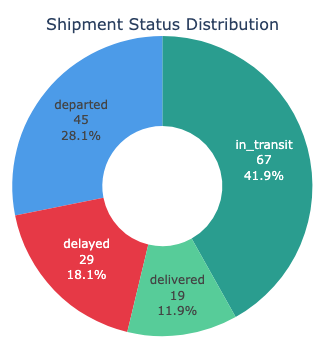
Figure 1. Shipment Status Distribution
Row 2 – Warehouse View
- Delayed shipments by warehouse: Which warehouses are handling the most delayed shipments right now
- Warehouse health score: A heatmap scoring each warehouse from 0.0 (everything delayed) to 1.0 (fully healthy), colored red through orange to green, as shown in Figure 2
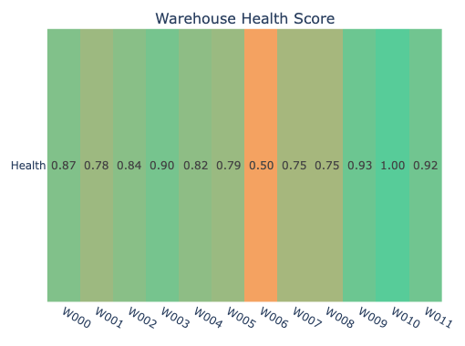
Figure 2. Warehouse Health Score
Row 3 – Origin and Destination
- Supplier performance: Which suppliers are generating the most delayed shipments
- Retailer impact: Which retailers are receiving the most delayed shipments — the downstream effect of any disruption
Row 4 – Mid-Network and Flow
- Average delay by distribution center: Where in the middle layer delays are accumulating
- Shipment flow: A Sankey diagram (Figure 3) showing which suppliers are routing through which warehouses
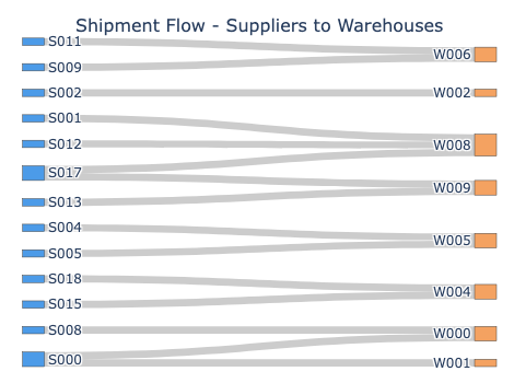
Figure 3. Shipment Flow - Suppliers to Warehouses
The warehouse health score is the most immediately readable panel. The Cypher behind it computes the score directly in the graph:
MATCH (sh:Shipment)-[:VIA_WAREHOUSE]->(w:Warehouse)
WHERE w.active IS NULL OR w.active <> false
WITH w.id AS warehouse,
     count(sh) AS total,
     count(CASE WHEN sh.status = 'delayed' THEN 1 END) AS delayed
RETURN warehouse,
       round(1.0 - toFloat(delayed) / total, 3) AS health_score
ORDER BY warehouse
Simulating a Network Disruption
One of the more compelling features of the graph model is how easy it is to simulate and visualize a disruption. Setting active = false on any node excludes it from the dashboard queries and the dashboard immediately reflects the simulated disruption on the next refresh cycle.
We can do this before the dashboard starts:
REMOVE_NODE = "W007" # mark this warehouse as inactiveOr live, while the dashboard is running, using the Neo4j AuraDB Query tab:
// Disable a node
MATCH (n {id: "W007"})
SET n.active = false

// Re-enable a node
MATCH (n {id: "W007"})
REMOVE n.active

// Check what is currently disabled
MATCH (n) WHERE n.active = false
RETURN labels(n)[0] AS label, n.id AS id
Within 5 seconds, the dashboard reflects the change. The warehouse health heatmap shows the gap, the delayed shipments bar shifts to other warehouses as traffic reroutes, and the network status table shows the node as disabled. Re-enabling it and watching the metrics recover completes the disruption and recovery story.
Standalone Operation
At startup, the consumer notebook creates the supply chain nodes using MERGE. This operation is idempotent, so any existing nodes from the previous article are left unchanged. Note that this step creates nodes only — the relationships between supply chain nodes (supplier -> warehouse -> distribution center -> retailer) are assumed to exist from the previous article, or can be added separately if running this notebook in isolation.
with driver.session(database = NEO4J_DATABASE) as session:
    for i in range(20):
        session.run("MERGE (:Supplier {id: $id})", id = f"S{i:03d}")
    for i in range(12):
        session.run("MERGE (:Warehouse {id: $id})", id = f"W{i:03d}")
    for i in range(10):
        session.run("MERGE (:DistributionCenter {id: $id})", id = f"DC{i:03d}")
    for i in range(30):
        session.run("MERGE (:Retailer {id: $id})", id = f"R{i:03d}")
Gotchas and Lessons Learned
Suppress librdkafka Logging
Without "log_level": 0 in the producer and consumer config, Confluent's underlying librdkafka library prints telemetry messages to the cell output every time a connection is established. The messages are harmless.
Suppress Neo4j Property Warnings
Querying a property that does not yet exist on any node produces a GqlStatusObject warning from Neo4j for every query that references it. The active property falls into this category when no node has been disabled. The fix is one line to set notifications to "OFF" on the driver, as follows:
driver = GraphDatabase.driver(
    NEO4J_URI,
    auth = (NEO4J_USERNAME, NEO4J_PASSWORD),
    notifications_min_severity = "OFF",
)
Consumer Group Isolation
Kafka distributes partitions across consumers in the same group, so each consumer processes only its assigned partitions. If we run multiple consumers using the same group ID against the same topic, each will only process a subset of the events. The dashboard uses supply-chain-dashboard as its group ID, and the tip is to run only one instance of this notebook at a time against the same topic and cluster.
auto.offset.reset = earliest
Without this setting, a consumer that starts after events have been published will miss everything that arrived before it connected. Setting earliest means the consumer always catches up on the full history of the topic before going live, which is essential if we stop and restart the dashboard mid-session.
Clear Shipment Nodes Between Runs
Each run of the consumer creates new Shipment nodes. Since the producer generates synthetic demo data, it's safe to clear these between runs; otherwise, successive runs would accumulate all historical shipments, and the dashboard counts would grow unbounded. The notebook clears all Shipment nodes at startup:
MATCH (sh:Shipment)
CALL (sh) { DETACH DELETE sh }
IN TRANSACTIONS OF 10000 ROWS
Summary
We've built a real-time supply chain event streaming pipeline using Confluent Cloud Kafka and Neo4j. The producer generates synthetic shipment events continuously, the consumer writes them into the graph, and a live dashboard shows network health updating in near real-time. The disruption simulation — marking a node inactive mid-run and watching the dashboard respond — demonstrates one of the most compelling aspects of the graph model: the ability to ask structural questions about a network as it evolves. The same architecture adapts naturally to real logistics, IoT, or manufacturing event streams where understanding network structure matters as much as raw throughput.
The full source code is available on GitHub.
Opinions expressed by DZone contributors are their own.
Comments