Machine Learning With Python: Data Preprocessing Techniques

Machine learning continues to be one of the most rapidly advancing and in-demand fields of technology. Machine learning, a branch of artificial intelligence, enables computer systems to learn and adopt human-like qualities, ultimately leading to the development of artificially intelligent machines. Eight key human-like qualities that can be imparted to a computer using machine learning as part of the field of artificial intelligence are presented in the table below.

However, the process of creating artificial intelligence requires large volumes of data. In machine learning, the more data that we have and train the model on, the better the model (AI agent) becomes at processing the given prompts or inputs and ultimately doing the task(s) for which it was trained.

This data is not fed into the machine learning algorithms in its raw form. It (the data) must first undergo various inspections and phases of data cleansing and preparation before it is fed into the learning algorithms. We call this phase of the machine learning life cycle, the data preprocessing phase. As implied by the name, this phase consists of all the operations and procedures that will be applied to our dataset (rows/columns of values) to bring it into a cleaned state so that it will be accepted by the machine learning algorithm to start the training/learning process.

This article will discuss and look at the most popular data preprocessing techniques used for machine learning. We will explore various methods to clean, transform, and scale our data. All exploration and practical examples will be done using Python code snippets to guide you with hands-on experience on how these techniques can be implemented effectively for your machine learning project.

Why Preprocess Data?

The literal holistic reason for preprocessing data is so that the data is accepted by the machine learning algorithm and thus, the training process can begin. However, if we look at the intrinsic inner workings of the machine learning framework itself, more reasons can be provided. The table below discusses the 5 key reasons (advantages) for preprocessing your data for the subsequent machine learning task.

In its raw state, data can have a magnitude of errors and noise in it. Data preprocessing seeks to clean and free the data from these errors. Common challenges that are experienced with raw data include, but are not limited to, the following:

• Missing values: Null values or NaN (Not-a-Number)
• Noisy data: Outliers or incorrectly captured data points
• Inconsistent data: Different data formatting inside the same file
• Imbalanced data: Unequal class distributions (experienced in classification tasks)

In the following sections of this article, we will proceed to work with hands-on examples of Data Preprocessing.

Data Preprocessing Techniques in Python

The frameworks that we will utilize to work with practical examples of data preprocessing:

NumPy

Pandas

SciKit Learn

Handling Missing Values

The most popular techniques to handle missing values are removal and imputation. It is interesting to note that irrespective of what operation you are trying to perform if there is at least one null (NaN) inside your calculation or process, then the entire operation will fail and evaluate to a NaN (null/missing/error) value.

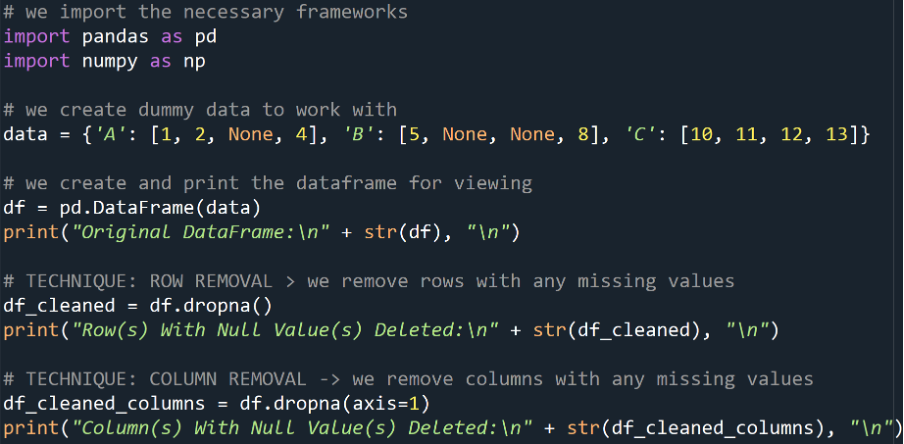
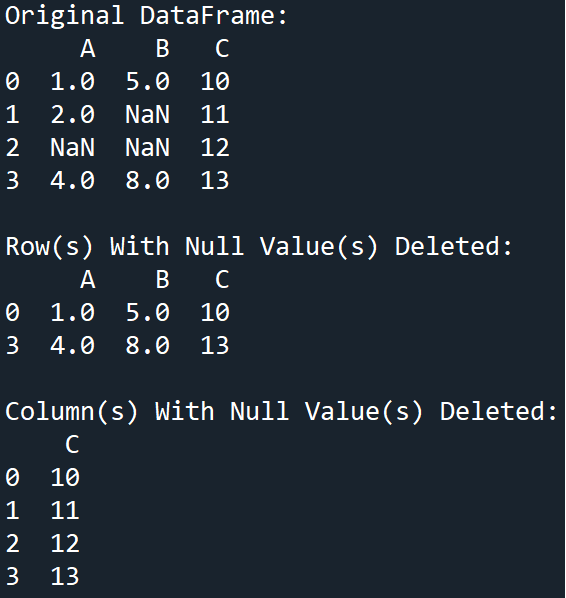
Removal

This is when we remove the rows or columns that contain the missing value(s). This is typically done when the proportion of missing data is relatively small compared to the entire dataset.

Example

Output

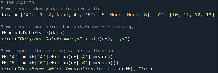
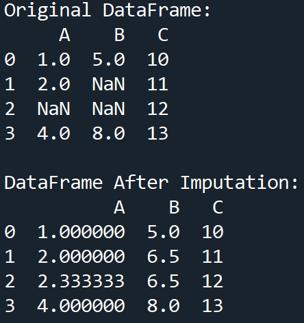
Imputation

This is when we replace the missing values in our data, with substituted values. The substituted value is commonly the mean, median, or mode of the data for that column. The term given to this process is imputation.

Example

Output

Handling Noisy Data

Our data is said to be noisy when we have outliers or irrelevant data points present. This noise can distort our model and therefore, our analysis. The common preprocessing techniques for handling noisy data include smoothing and binning.

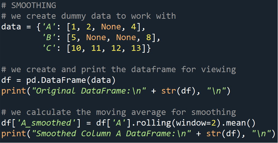
Smoothing

This data preprocessing technique involves employing operations such as moving averages to reduce noise and identify trends. This allows for the essence of the data to be encapsulated.

Example

Output

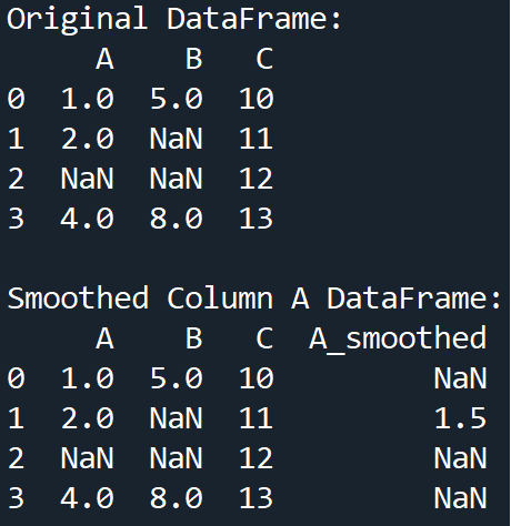
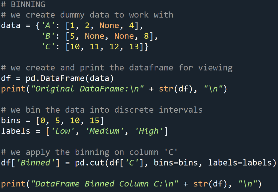
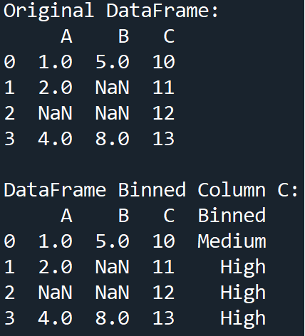
Binning

This is a common process in statistics and follows the same underlying logic in machine learning data preprocessing. It involves grouping our data into bins to reduce the effect of minor observation errors.

Example

Output

Data Transformation

This data preprocessing technique plays a crucial role in helping to shape and guide algorithms that require numerical features as input, to optimum training. This is because data transformation deals with converting our raw data into a suitable format or range for our machine learning algorithm to work with. It is a crucial step for distance-based machine learning algorithms.

The key data transformation techniques are normalization and standardization. As implied by the names of these operations, they are used to rescale the data within our features to a standard range or distribution.

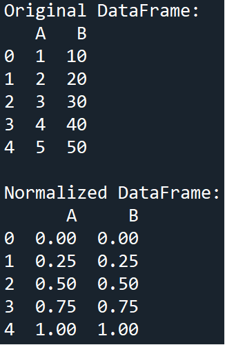
Normalization

This data preprocessing technique will scale our data to a range of [0, 1] (inclusive of both numbers) or [-1, 1] (inclusive of both numbers). It is useful when our features have different ranges and we want to bring them to a common scale.

Example

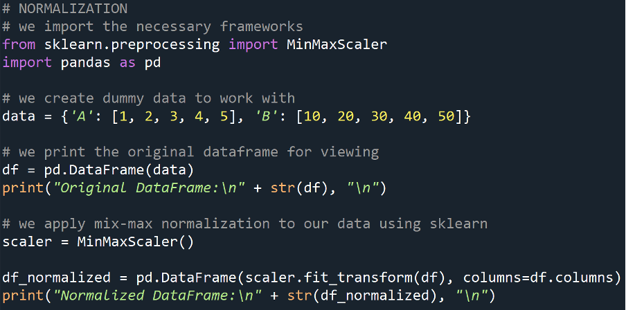
Output

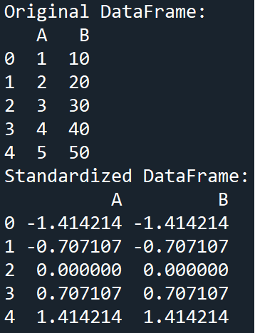
Standardization

Standardization will scale our data to have a mean of 0 and a standard deviation of 1. It is useful when the data contained within our features have different units of measurement or distribution.

Example

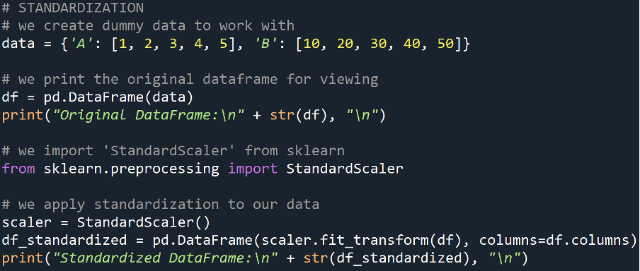
Output

Encoding Categorical Data

Our machine learning algorithms most often require the features matrix (input data) to be in the form of numbers, i.e., numerical/quantitative. However, our dataset may contain textual (categorical) data. Thus, all categorical (textual) data must be converted into a numerical format before feeding the data into the machine learning algorithm. The most commonly implemented techniques for handling categorical data include one-hot encoding (OHE) and label encoding.

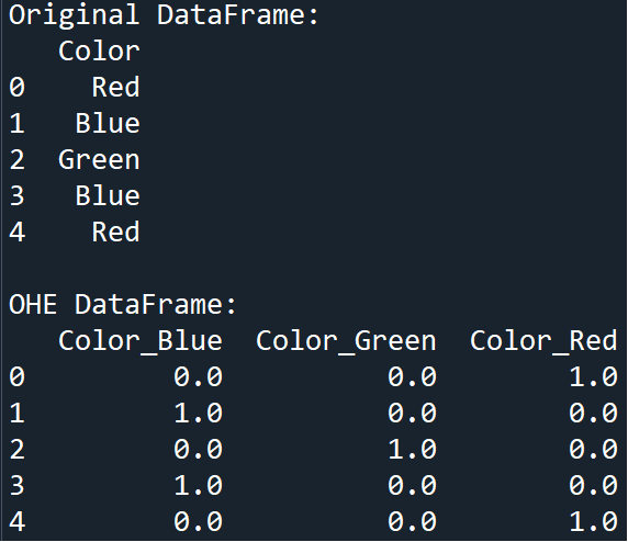
One-Hot Encoding

This data preprocessing technique is employed to convert categorical values into binary vectors. This means that each unique category becomes its column inside the data frame, and the presence of the observation (row) containing that value or not, is represented by a binary 1 or 0 in the new column.

Example

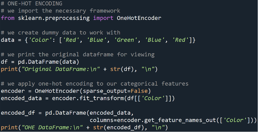
Output

Label Encoding

This is when our categorical values are converted into integer labels. Essentially, each unique category is assigned a unique integer to represent hitherto.

Example

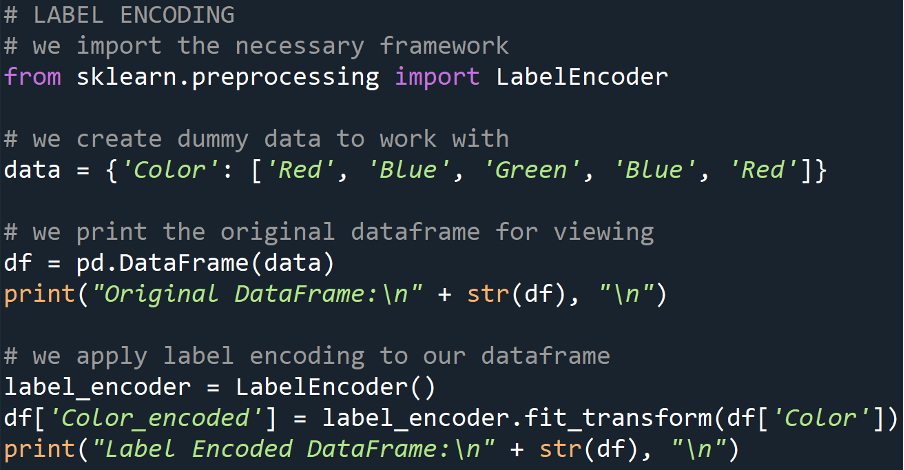
Output

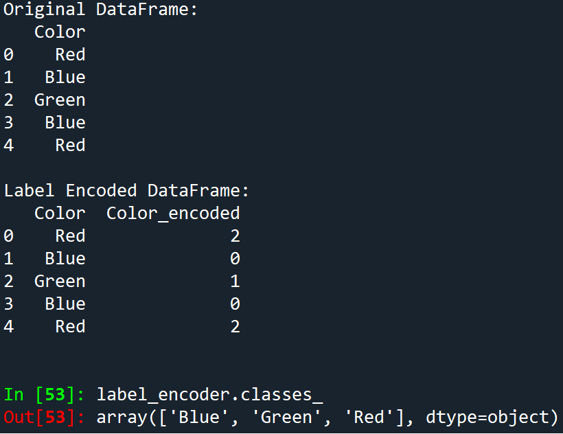
This tells us that the label encoding was done as follows:

• ‘Blue’ -> 0
• ‘Green’ -> 1
• ‘Red’ -> 2

P.S., the numerical assignment is Zero-Indexed (as with all collection types in Python)

Feature Extraction and Selection

As implied by the name of this data preprocessing technique, feature extraction/selection involves the machine learning practitioner selecting the most important features from the data, while feature extraction transforms the data into a reduced set of features.

Feature Selection

This data preprocessing technique helps us in identifying and selecting the features from our dataset that have the most significant impact on the model. Ultimately, selecting the best features will improve the performance of our model and reduce overfitting thereof.

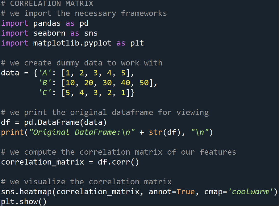
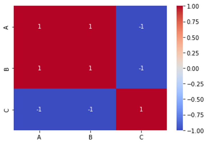
Correlation Matrix

This is a matrix that helps us identify features that are highly correlated thereby allowing us to remove redundant features. “The correlation coefficients range from -1 to 1, where values closer to -1 or 1 indicate stronger correlation, while values closer to 0 indicate weaker or no correlation”.

Example

Output 1

Output 2

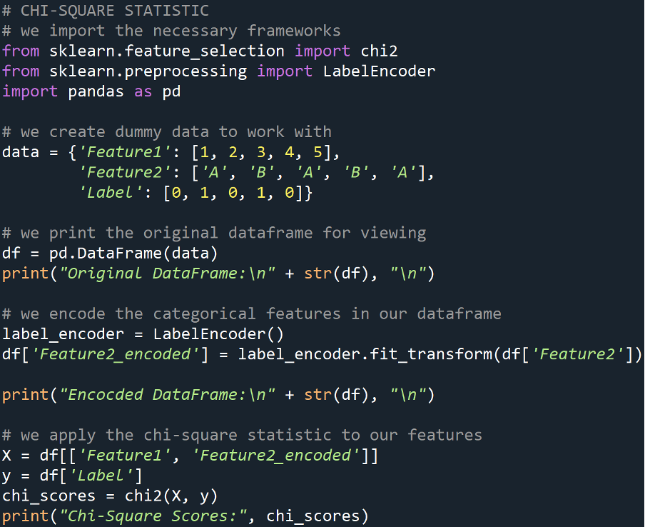
Chi-Square Statistic

The Chi-Square Statistic is a test that measures the independence of two categorical variables. It is very useful when we are performing feature selection on categorical data. It calculates the p-value for our features which tells us how useful our features are for the task at hand.

Example

Output

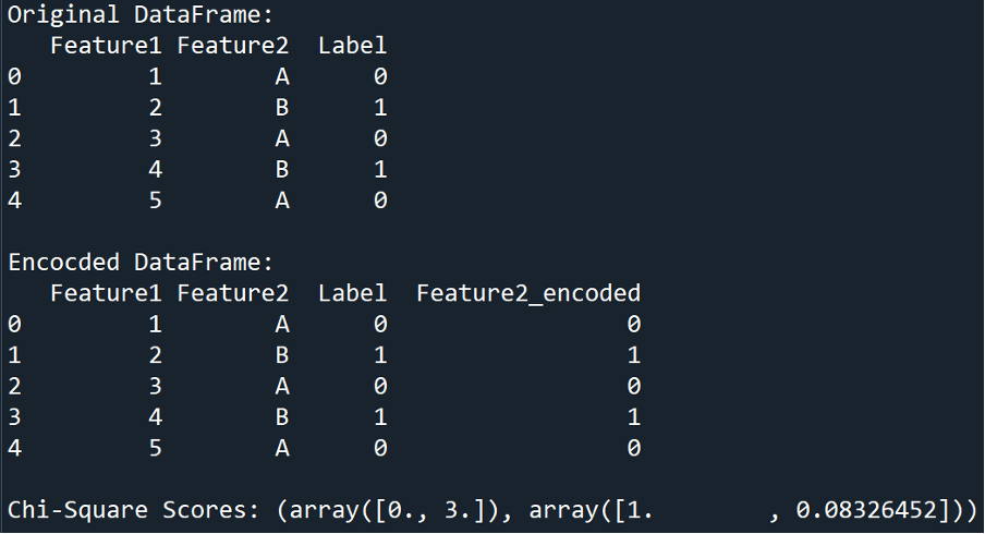
The output of the Chi-Square scores consists of two arrays:

• The first array contains the Chi-Square statistic values for each feature.
• The second array contains the p-values corresponding to each feature.

In our example:

• For the first feature:
  1. The chi-square statistic value is 0.0
  2. p-value is 1.0
• For the second feature:
  1. The chi-square statistic value is 3.0
  2. p-value is approximately 0.083

The Chi-Square statistic measures the association between the feature and the target variable. A higher Chi-Square value indicates a stronger association between the feature and the target. This tells us that the feature being analyzed is very useful in guiding the model to the desired target output.

The p-value measures the probability of observing the Chi-Square statistic under the null hypothesis that the feature and the target are independent. Essentially, A low p-value (typically < 0.05) indicates that the association between the feature and the target is statistically significant.

For our first feature, the Chi-Square value is 0.0, and the p-value is 1.0 thereby indicating no association with the target variable.

For the second feature, the Chi-Square value is 3.0, and the corresponding p-value is approximately 0.083. This suggests that there might be some association between our second feature and the target variable. Keep in mind that we are working with dummy data and in the real world, the data will give you a lot more variation and points of analysis.

Feature Extraction

This is a data preprocessing technique that allows us to reduce the dimensionality of the data by transforming it into a new set of features. Logically speaking, model performance can be drastically increased by employing feature selection and extraction techniques.

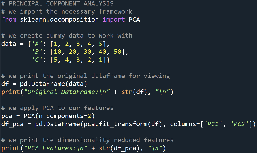
Principal Component Analysis (PCA)

PCA is a data preprocessing dimensionality reduction technique that transforms our data into a set of right-angled (orthogonal) components thereby capturing the most variance present in our features.

Example

Output

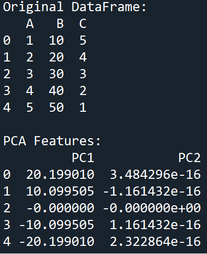
With this, we have successfully explored a variety of the most commonly used data preprocessing techniques that are used in Python machine learning tasks.

Conclusion

In this article, we explored popular data preprocessing techniques for machine learning with Python. We began by understanding the importance of data preprocessing and then looked at the common challenges associated with raw data. We then dove into various preprocessing techniques with hands-on examples in Python.

Ultimately, data preprocessing is a step that cannot be skipped from your machine learning project lifecycle. Even if there are no changes or transformations to be made to your data, it is always worth the effort to apply these techniques to your data where applicable. because, in doing so, you will ensure that your data is cleaned and transformed for your machine learning algorithm and thus your subsequent machine learning model development factors such as model accuracy, computational complexity, and interpretability will see an improvement.

In conclusion, data preprocessing lays the foundation for successful machine-learning projects. By paying attention to data quality and employing appropriate preprocessing techniques, we can unlock the full potential of our data and build models that deliver meaningful insights and actionable results.

Code

# -*- coding: utf-8 -*-
"""
@author: Karthik Rajashekaran
"""

# we import the necessary frameworks
import pandas as pd
import numpy as np

# we create dummy data to work with
data = {'A': [1, 2, None, 4], 'B': [5, None, None, 8], 'C': [10, 11, 12, 13]}

# we create and print the dataframe for viewing
df = pd.DataFrame(data)
print("Original DataFrame:\n" + str(df), "\n")

# TECHNIQUE: ROW REMOVAL > we remove rows with any missing values
df_cleaned = df.dropna()
print("Row(s) With Null Value(s) Deleted:\n" + str(df_cleaned), "\n")

# TECHNIQUE: COLUMN REMOVAL -> we remove columns with any missing values
df_cleaned_columns = df.dropna(axis=1)
print("Column(s) With Null Value(s) Deleted:\n" + str(df_cleaned_columns), "\n")

#%%
# IMPUTATION
# we create dummy data to work with
data = {'A': [1, 2, None, 4], 'B': [5, None, None, 8], 'C': [10, 11, 12, 13]}

# we create and print the dataframe for viewing
df = pd.DataFrame(data)
print("Original DataFrame:\n" + str(df), "\n")

# we impute the missing values with mean
df['A'] = df['A'].fillna(df['A'].mean())
df['B'] = df['B'].fillna(df['B'].median())
print("DataFrame After Imputation:\n" + str(df), "\n")

#%%
# SMOOTHING
# we create dummy data to work with
data = {'A': [1, 2, None, 4],
        'B': [5, None, None, 8],
        'C': [10, 11, 12, 13]}

# we create and print the dataframe for viewing
df = pd.DataFrame(data)
print("Original DataFrame:\n" + str(df), "\n")

# we calculate the moving average for smoothing
df['A_smoothed'] = df['A'].rolling(window=2).mean()
print("Smoothed Column A DataFrame:\n" + str(df), "\n")

#%%
# BINNING
# we create dummy data to work with
data = {'A': [1, 2, None, 4],
        'B': [5, None, None, 8],
        'C': [10, 11, 12, 13]}

# we create and print the dataframe for viewing
df = pd.DataFrame(data)
print("Original DataFrame:\n" + str(df), "\n")

# we bin the data into discrete intervals
bins = [0, 5, 10, 15]
labels = ['Low', 'Medium', 'High']

# we apply the binning on column 'C'
df['Binned'] = pd.cut(df['C'], bins=bins, labels=labels)

print("DataFrame Binned Column C:\n" + str(df), "\n")

#%%
# NORMALIZATION
# we import the necessary frameworks
from sklearn.preprocessing import MinMaxScaler
import pandas as pd

# we create dummy data to work with
data = {'A': [1, 2, 3, 4, 5], 'B': [10, 20, 30, 40, 50]}

# we print the original dataframe for viewing
df = pd.DataFrame(data)
print("Original DataFrame:\n" + str(df), "\n")

# we apply mix-max normalization to our data using sklearn
scaler = MinMaxScaler()

df_normalized = pd.DataFrame(scaler.fit_transform(df), columns=df.columns)
print("Normalized DataFrame:\n" + str(df_normalized), "\n")

#%%
# STANDARDIZATION
# we create dummy data to work with
data = {'A': [1, 2, 3, 4, 5], 'B': [10, 20, 30, 40, 50]}

# we print the original dataframe for viewing
df = pd.DataFrame(data)
print("Original DataFrame:\n" + str(df), "\n")

# we import 'StandardScaler' from sklearn
from sklearn.preprocessing import StandardScaler

# we apply standardization to our data
scaler = StandardScaler()
df_standardized = pd.DataFrame(scaler.fit_transform(df), columns=df.columns)
print("Standardized DataFrame:\n" + str(df_standardized), "\n")

#%%
# ONE-HOT ENCODING
# we import the necessary framework
from sklearn.preprocessing import OneHotEncoder

# we create dummy data to work with
data = {'Color': ['Red', 'Blue', 'Green', 'Blue', 'Red']}

# we print the original dataframe for viewing
df = pd.DataFrame(data)
print("Original DataFrame:\n" + str(df), "\n")

# we apply one-hot encoding to our categorical features
encoder = OneHotEncoder(sparse_output=False)
encoded_data = encoder.fit_transform(df[['Color']])

encoded_df = pd.DataFrame(encoded_data,
                          columns=encoder.get_feature_names_out(['Color']))
print("OHE DataFrame:\n" + str(encoded_df), "\n")

#%%
# LABEL ENCODING
# we import the necessary framework
from sklearn.preprocessing import LabelEncoder

# we create dummy data to work with
data = {'Color': ['Red', 'Blue', 'Green', 'Blue', 'Red']}

# we print the original dataframe for viewing
df = pd.DataFrame(data)
print("Original DataFrame:\n" + str(df), "\n")

# we apply label encoding to our dataframe
label_encoder = LabelEncoder()
df['Color_encoded'] = label_encoder.fit_transform(df['Color'])
print("Label Encoded DataFrame:\n" + str(df), "\n")

#%%
# CORRELATION MATRIX
# we import the necessary frameworks
import pandas as pd
import seaborn as sns
import matplotlib.pyplot as plt

# we create dummy data to work with
data = {'A': [1, 2, 3, 4, 5],
        'B': [10, 20, 30, 40, 50],
        'C': [5, 4, 3, 2, 1]}

# we print the original dataframe for viewing
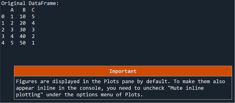
df = pd.DataFrame(data)
print("Original DataFrame:\n" + str(df), "\n")

# we compute the correlation matrix of our features
correlation_matrix = df.corr()

# we visualize the correlation matrix
sns.heatmap(correlation_matrix, annot=True, cmap='coolwarm')
plt.show()

#%%
# CHI-SQUARE STATISTIC
# we import the necessary frameworks
from sklearn.feature_selection import chi2
from sklearn.preprocessing import LabelEncoder
import pandas as pd

# we create dummy data to work with
data = {'Feature1': [1, 2, 3, 4, 5],
        'Feature2': ['A', 'B', 'A', 'B', 'A'],
        'Label': [0, 1, 0, 1, 0]}

# we print the original dataframe for viewing
df = pd.DataFrame(data)
print("Original DataFrame:\n" + str(df), "\n")

# we encode the categorical features in our dataframe
label_encoder = LabelEncoder()
df['Feature2_encoded'] = label_encoder.fit_transform(df['Feature2'])

print("Encocded DataFrame:\n" + str(df), "\n")

# we apply the chi-square statistic to our features
X = df[['Feature1', 'Feature2_encoded']]
y = df['Label']
chi_scores = chi2(X, y)
print("Chi-Square Scores:", chi_scores)

#%%
# PRINCIPAL COMPONENT ANALYSIS
# we import the necessary framework
from sklearn.decomposition import PCA

# we create dummy data to work with
data = {'A': [1, 2, 3, 4, 5],
        'B': [10, 20, 30, 40, 50],
        'C': [5, 4, 3, 2, 1]}

# we print the original dataframe for viewing
df = pd.DataFrame(data)
print("Original DataFrame:\n" + str(df), "\n")

# we apply PCA to our features
pca = PCA(n_components=2)
df_pca = pd.DataFrame(pca.fit_transform(df), columns=['PC1', 'PC2'])

# we print the dimensionality reduced features
print("PCA Features:\n" + str(df_pca), "\n")

References

Datacamp, How to Learn Machine Learning in 2024, February 2024. [Online]. [Accessed: 30 May 2024].

Statista, Growth of worldwide machine learning (ML) market size from 2021 to 2030, 13 February 2024. [Online]. [Accessed: 30 May 2024].

Hurne M.v., What is affective computing/emotion AI? 03 May 2024. [Online]. [Accessed: 30 May 2024].