Building a Feature Store With Neo4j and Feast

Feature stores solve a problem that every machine learning (ML) team eventually hits: the features you compute during training are different from the ones you retrieve at serving time. Feast is an open-source feature store that bridges that gap, handling the registry, materialization, and online retrieval so a model sees the same data in production as it did during training.

Often, Feast tutorials pair it with a relational database or a cloud data warehouse. In this article, we'll do something different. We'll use Neo4j Desktop as the feature computation engine. Five features are ordinary aggregations that Cypher handles as easily as SQL. The sixth, a customer community_id, comes from graph algorithms: customers with similar purchase mixes are found with Graph Data Science (GDS) node similarity and then grouped with Louvain community detection. We'll hand all six features to Feast, which materializes them into a SQLite online store, serves them at inference time, and builds point-in-time correct training data.

We'll also test, on held-out orders, whether the graph feature tells a model anything that a plain favorite_category column doesn't.

The full source code is available on GitHub.

Architecture

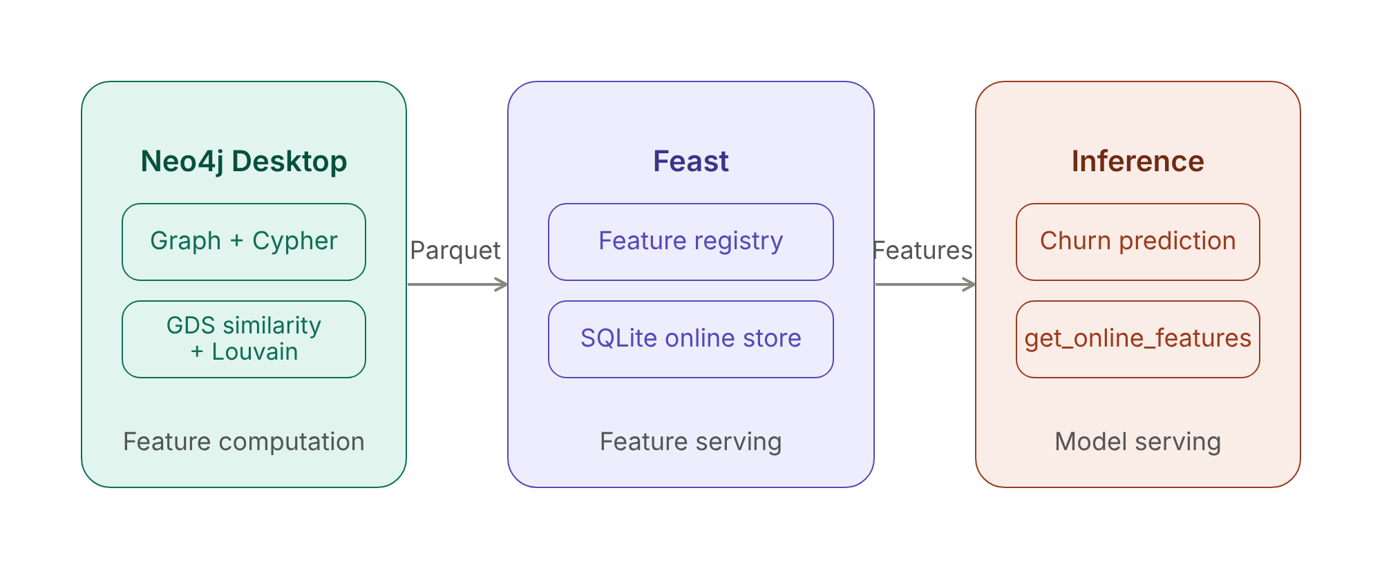
Figure 1. Architecture

As shown in Figure 1, the architecture has three layers. Neo4j Desktop handles feature computation: standard aggregations via Cypher and a graph-native community feature via the Graph Data Science (GDS) library. The results, computed at several points in time, land in a Parquet file, which acts as Feast's offline store. Feast then materializes the latest values from Parquet into SQLite for low-latency online serving. At inference time, a single get_online_features() call retrieves the full feature vector, regardless of whether a feature came from a Cypher query or a GDS algorithm. For training data, get_historical_features() reads the same offline store.

The key insight is that Feast doesn't know or care how the Parquet file was produced.

What We're Building

We'll work with a synthetic e-commerce dataset of 100 customers, 3,000 orders, and 5 product categories (Electronics, Clothing, Home, Books, and Sports) spread over the last 90 days. Each customer belongs to a hidden segment defined by a primary and a secondary category. For 55% of their orders the category is the segment's primary one, for 30% it is the secondary one, and for the remaining 15% it is drawn uniformly from all five categories. There are five segments:

• Electronics (primary) and Home (secondary)
• Electronics and Sports
• Clothing and Books
• Clothing and Home
• Books and Sports

The design is deliberate. Two segments share Electronics as their primary category and two share Clothing, so a customer's single most-bought category can't tell those segments apart. Only the combination of categories can. To make the churn example meaningful, 18 customers are also made to go quiet: 8 have not ordered for more than 60 days and 10 for more than 30 days.

The segment is stored on each Customer node, but only so we can check our results later. It is never used to compute any feature.

We'll compute six features per customer, as of a given date:

• total_orders – Number of orders placed up to the as-of date
• total_spent – Total order value
• avg_order_value – Mean order value
• days_since_last_order – Recency, measured from the as-of date
• favorite_category – The category with the most orders
• community_id – Graph-native feature from node similarity and Louvain community detection

We compute them at three as-of dates (60 days ago, 30 days ago, and today), so that Feast can later reconstruct what was known at any point in time.

Setup

A virtual environment is highly recommended. For example:

python3 -m venv ~/feast-env
source ~/feast-env/bin/activate

The notebook was run against Neo4j 2026.07.0 (Enterprise) and GDS 2026.07.0.

We need Neo4j Desktop running with the Graph Data Science (GDS) plugin installed. In Neo4j Desktop, go to Plugins and install the Graph Data Science Library. Credentials go in environment variables before running the Jupyter notebook:

export NEO4J_URI="bolt://localhost:7687"
export NEO4J_USERNAME="neo4j"
export NEO4J_PASSWORD="your-password"
export NEO4J_DATABASE="your-database"

Warning: The notebook removes all data, indexes, and constraints from the database named in NEO4J_DATABASE before loading its sample data. Use a database you are happy to wipe.

We'll connect to Neo4j with the standard driver:

driver = GraphDatabase.driver(
    NEO4J_URI,
    auth = (NEO4J_USERNAME, NEO4J_PASSWORD)
)

Feature Definitions

Feast needs two files: a project config and a feature view declaration.

The config points to SQLite for the online store:

project: ecommerce_features
registry: feature_repo/registry.db
provider: local

online_store:
    type: sqlite
    path: feature_repo/online_store.db

The feature definitions declare the customer_id entity and a feature view with all six features, including community_id as an Int64:

from feast import Entity, FeatureView, Field, FileSource
from feast.types import Float32, Int64, String, ValueType
from datetime import timedelta

customer = Entity(
    name = "customer_id",
    description = "Customer identifier",
    value_type = ValueType.STRING
)

customer_features = FeatureView(
    name = "customer_features",
    entities = [customer],
    ttl = timedelta(days = 90),
    schema = [
        Field(name = "total_orders",          dtype = Int64),
        Field(name = "total_spent",           dtype = Float32),
        Field(name = "avg_order_value",       dtype = Float32),
        Field(name = "days_since_last_order", dtype = Int64),
        Field(name = "favorite_category",     dtype = String),
        Field(name = "community_id",          dtype = Int64),
    ],
    online = True,
    source = FileSource(
        path = "data/customer_features.parquet",
        timestamp_field = "event_timestamp"
    ),
)

From Feast's perspective, community_id is just another integer column. It doesn't know it took graph algorithms to produce it.

Loading Data into Neo4j

Rather than rows in a table, we'll model the data as a graph. Figure 2 shows the structure.

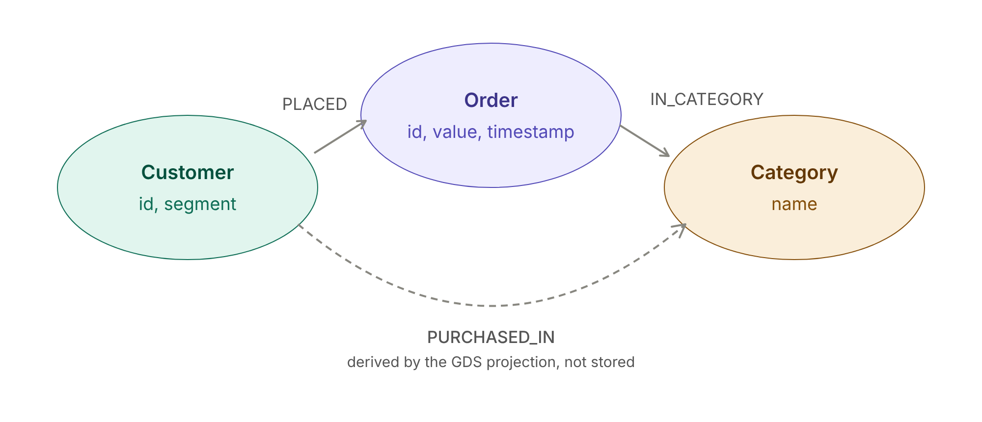
Figure 2. Graph Data Model

Customer and Order nodes connect via PLACED relationships. Each Order connects to a Category node via IN_CATEGORY. We don't store a direct customer-to-category relationship. Instead, the GDS projection derives one at query time, so that it can be limited to orders placed before a given date. All timestamps are timezone-aware (UTC).

UNWIND $orders AS o
MERGE (c:Customer {id: o.customer_id})
  ON CREATE SET c.segment = o.segment
MERGE (cat:Category {name: o.product_category})
CREATE (ord:Order {
    id:        o.order_id,
    value:     o.order_value,
    timestamp: datetime(o.order_timestamp),
    quantity:  o.quantity
})
MERGE (c)-[:PLACED]->(ord)
MERGE (ord)-[:IN_CATEGORY]->(cat)

Standard Features via Cypher

The first five features come from two Cypher queries, both limited to orders placed on or before the as-of date $as_of. The main aggregation computes counts, totals, averages, and recency in a single pass:

MATCH (c:Customer)-[:PLACED]->(o:Order)
WHERE o.timestamp <= datetime($as_of)
RETURN
    c.id         AS customer_id,
    count(o)     AS total_orders,
    sum(o.value) AS total_spent,
    avg(o.value) AS avg_order_value,
    duration.inDays(max(o.timestamp), datetime($as_of)).days AS days_since_last_order

Favorite category requires a separate query, since we need to find the top category per customer and collect() the first result after ordering. Ties are broken alphabetically so that the result is deterministic:

MATCH (c:Customer)-[:PLACED]->(o:Order)-[:IN_CATEGORY]->(cat:Category)
WHERE o.timestamp <= datetime($as_of)
WITH c.id AS customer_id, cat.name AS category, count(*) AS cnt
ORDER BY customer_id, cnt DESC, category
WITH customer_id, collect(category)[0] AS favorite_category
RETURN customer_id, favorite_category

The event_timestamp that Feast uses is the as-of date itself. In other words, the moment the features describe, rather than the time of the customer's last order.

Graph-Native Feature: Community ID

The sixth feature groups customers whose purchase mixes are similar. It takes four steps, all run inside Neo4j.

Step 1: Project customers and categories. We use the current Cypher projection, which builds an in-memory graph with the gds.graph.project aggregation function and replaces the deprecated gds.graph.project.cypher procedure. Each customer-category relationship is weighted by the number of orders placed up to the as-of date:

MATCH (c:Customer)-[:PLACED]->(o:Order)-[:IN_CATEGORY]->(cat:Category)
WHERE o.timestamp <= datetime($as_of)
WITH c, cat, count(o) AS order_count
WITH gds.graph.project(
    $name, c, cat,
    {
        sourceNodeLabels:       labels(c),
        targetNodeLabels:       labels(cat),
        relationshipType:       'PURCHASED_IN',
        relationshipProperties: {order_count: order_count}
    }
) AS g
RETURN g.graphName AS graph, g.nodeCount AS nodes, g.relationshipCount AS relationships

Step 2: Find similar customers. GDS node similarity with the cosine metric, weighted by order count, scores two customers close to 1 when their category mixes point in the same direction. We keep each customer's 15 most similar customers above a cutoff of 0.8:

CALL gds.nodeSimilarity.stream($name, $config)
YIELD node1, node2, similarity
RETURN gds.util.asNode(node1).id AS src,
       gds.util.asNode(node2).id AS dst,
       similarity

config = {
    "similarityMetric":           "COSINE",
    "relationshipWeightProperty": "order_count",
    "topK":                       SIMILARITY_TOP_K,
    "similarityCutoff":           SIMILARITY_CUTOFF,
}

Step 3: Project a customer-to-customer graph from those pairs, weighted by similarity:

UNWIND $pairs AS p
MATCH (a:Customer {id: p.src}), (b:Customer {id: p.dst})
WITH gds.graph.project(
    $name, a, b,
    {
        sourceNodeLabels:       labels(a),
        targetNodeLabels:       labels(b),
        relationshipType:       'SIMILAR',
        relationshipProperties: {similarity: p.similarity}
    },
    {undirectedRelationshipTypes: ['*']}
) AS g
RETURN g.graphName AS graph, g.nodeCount AS nodes, g.relationshipCount AS relationships

Step 4: Run Louvain on that graph, using the similarity scores as relationship weights. consecutiveIds gives us small, tidy community IDs:

CALL gds.louvain.stream($name, $config)
YIELD nodeId, communityId
WITH gds.util.asNode(nodeId) AS n, communityId
WHERE n:Customer
RETURN n.id AS customer_id, communityId AS community_id

A customer with no sufficiently similar neighbor isn't in the similarity graph, so we give each such customer a community of their own. The two settings, SIMILARITY_TOP_K (15) and SIMILARITY_CUTOFF (0.8), are the only knobs, and we didn't tune them.

Why not run Louvain directly on the customer-category graph and skip the similarity step? We tried, and the next section shows why we didn't keep it.

Which Grouping Recovers the Hidden Segments?

We compared four ways of grouping the same customers against the hidden segments, using the Adjusted Rand Index (ARI), where 1.0 means identical groupings and values near 0 mean no better than chance:

Grouping                                                Groups    ARI vs hidden segments
----------------------------------------------------  --------  ------------------------
1. favorite_category                                         5                      0.52
2. Louvain, customer-category graph, unweighted              2                      0.08
3. Louvain, customer-category graph, weighted                3                      0.41
4. Louvain, customer-similarity graph (community_id)         5                      0.98

A plain favorite_category scores 0.52. It can't separate segments that share a primary category and the cross-tabulation shows exactly that: Electronics lumps together 21 customers from one segment and 22 from another and Clothing does the same with 20 and 15.

favorite_category vs hidden segment (latest snapshot):
segment            Books + Sports  Clothing + Books  Clothing + Home  Electronics + Home  Electronics + Sports
favorite_category                                                                                             
Books                          14                 2                0                   0                     0
Clothing                        0                20               15                   0                     0
Electronics                     0                 0                0                  21                    22
Home                            0                 0                0                   2                     0
Sports                          2                 0                0                   0                     2

Louvain run directly on the customer-category graph does worse than that, with an ARI of 0.41 when weighted by order count and 0.08 when unweighted. We didn't investigate why, but the likely cause is that two segments sharing a primary category both attach to the same category node, which pulls them together. Without weights, every customer is linked to every category equally, and there is little left to separate them.

The similarity-graph method scores 0.98 and finds five communities that line up with the five segments:

community_id vs hidden segment (latest snapshot):
segment       Books + Sports  Clothing + Books  Clothing + Home  Electronics + Home  Electronics + Sports
community_id                                                                                             
0                          0                 0                0                  23                     0
1                          0                 1               15                   0                     0
2                          0                21                0                   0                     0
3                          0                 0                0                   0                    24
4                         16                 0                0                   0                     0

Figure 3 shows the five communities, each labeled with the segment that makes up most of it.

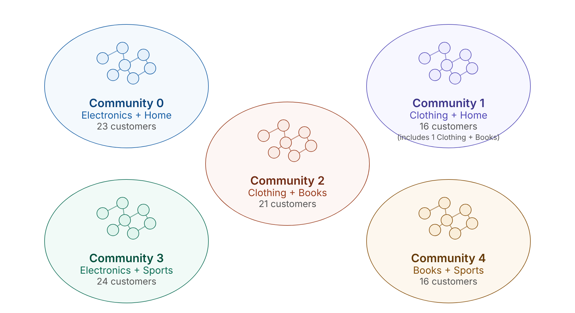
Figure 3. Communities Found by Node Similarity and Louvain.

Only one customer lands in the wrong community. The algorithm was never given the segments, so it recovered them from purchase behavior alone.

Does the Community Feature Add Predictive Signal?

Recovering hidden segments is reassuring, but a feature earns its place by helping predictions. We test that without training a model, using only the features as they were 30 days ago. For each group of customers, we estimate a mix of product categories from orders up to that date, then score how well that mix predicts the category of every order placed afterward. The score is log-loss, the average of the negative log of the probability given to the category actually bought, so lower is better. There is no leakage: both favorite_category and community_id were computed from orders placed before the cutoff.

def heldout_losses(orders, snapshot, cutoff_ts, group_col, alpha = 1.0):
    """How well does a grouping of customers predict the category of FUTURE orders?

    For each group, estimate the category mix from orders up to `cutoff_ts`
    (with add-`alpha` smoothing). Then score each later order by the negative log
    of the probability that mix gave its category. Lower is better.
    Returns one loss per held-out order."""

    groups = snapshot[["customer_id", group_col]].rename(columns = {group_col: "group"})
    train  = orders[orders["ts"] <= cutoff_ts].merge(groups, on = "customer_id")
    test   = orders[orders["ts"] >  cutoff_ts].merge(groups, on = "customer_id")

    counts = (train.groupby(["group", "category"]).size().unstack(fill_value = 0)
                   .reindex(columns = CATEGORIES, fill_value = 0) + alpha)
    probs  = counts.div(counts.sum(axis = 1), axis = 0)

    idx = pd.MultiIndex.from_arrays([test["group"], test["category"]])
    p   = probs.stack().reindex(idx).fillna(1 / len(CATEGORIES)).values

    return -np.log(p)

We compare no grouping at all, favorite_category, community_id and the hidden segment as an upper bound that no real feature could beat. A paired bootstrap gives a confidence interval for the improvement of community_id over favorite_category:

diff = losses["favorite_category"] - losses["community_id"]
rng  = np.random.default_rng(SEED)
boot = np.array([rng.choice(diff, size = len(diff), replace = True).mean() for _ in range(2000)])
low, high = np.percentile(boot, [2.5, 97.5])

Held-out orders (placed after the 30-day snapshot): 827

Grouping                                 Groups    Held-out log-loss (lower is better)
-------------------------------------  --------  -------------------------------------
No grouping (everyone shares one mix)         1                                  1.565
favorite_category                             5                                  1.171
community_id                                  5                                  1.025
Hidden segment (oracle upper bound)           5                                  1.009

Improvement of community_id over favorite_category: 0.146 (95% CI 0.110 to 0.180)

Grouping customers by favorite_category cuts the loss from 1.565 to 1.171. Grouping by community_id cuts it to 1.025, close to the 1.009 of the hidden segments. The improvement over favorite_category is 0.146, with a 95% confidence interval of 0.110 to 0.180. The reason is intuitive: knowing a customer's secondary category tells you what they are likely to buy after their favorite, and the community captures that while a single favorite category can't.

Some caveats apply. The data are synthetic and designed so the combination of categories matters, so the size of the gain reflects that design, not what you would see in real orders. The predictor is a simple count-based one rather than a trained model. The bootstrap resamples individual orders and ignores that orders from one customer are related, so the interval is somewhat optimistic. And this is one dataset from one random seed.

It is also worth saying what happened before we changed the data. In an earlier version of this example, every customer had a single preferred category. There, community_id and favorite_category agreed exactly (ARI 1.00), so the graph feature added nothing. The gain here appears when group membership depends on a combination of categories, which is the situation where a single aggregate column falls short.

Snapshots and Stable Community IDs

To support point-in-time retrieval, we compute all six features at three as-of dates: 60 days ago, 30 days ago, and today, and stack the results. Louvain runs independently for each date, and that creates a problem. Community IDs are arbitrary labels, and a label such as 3 in one run need not mean the same group in the next. A model trained on one snapshot would then be served IDs with a different meaning.

We solve this by relabeling each snapshot to match the previous one, assigning each new community the old ID it overlaps with most:

def align_communities(current, reference):
    """Relabel `current` community IDs to match `reference` by greatest member overlap."""

    merged = current[["customer_id", "community_id"]].merge(
        reference[["customer_id", "community_id"]],
        on = "customer_id", suffixes = ("_cur", "_ref")
    )
    overlap = (merged.groupby(["community_id_cur", "community_id_ref"])
                     .size().reset_index(name = "n")
                     .sort_values("n", ascending = False))

    mapping, used = {}, set()
    for _, r in overlap.iterrows():
        cur, ref = int(r["community_id_cur"]), int(r["community_id_ref"])
        if cur not in mapping and ref not in used:
            mapping[cur] = ref
            used.add(ref)

    # Any community with no counterpart in the reference gets a fresh ID
    next_id = int(max(reference["community_id"].max(), max(mapping.values(), default = -1))) + 1
    for cur in current["community_id"].unique():
        if int(cur) not in mapping:
            mapping[int(cur)] = next_id
            next_id += 1

    aligned = current.copy()
    aligned["community_id"] = aligned["community_id"].map(lambda x: mapping[int(x)]).astype("int64")
    return aligned

for days in SNAPSHOT_OFFSETS_DAYS:
    as_of = now - timedelta(days = days)
    df, stats = compute_features_as_of(as_of)

    if reference is not None:
        df = align_communities(df, reference)

    reference = df[["customer_id", "community_id"]]
    frames.append(df)

features_df = pd.concat(frames, ignore_index = True)

The notebook prints how well each snapshot recovers the segments and how much the labels would have disagreed without alignment:

As of 2026-08-27 (60 days ago): 100 customers, 844 similar pairs, 5 communities, ARI vs hidden segments 0.95
As of 2026-09-26 (30 days ago): 100 customers, 847 similar pairs, 5 communities, ARI vs hidden segments 0.95
    label agreement with previous snapshot: raw 65% -> aligned 96%
As of 2026-10-26 ( 0 days ago): 100 customers, 856 similar pairs, 5 communities, ARI vs hidden segments 0.98
    label agreement with previous snapshot: raw 63% -> aligned 99%

Each snapshot finds five communities and recovers the hidden segments well (ARI 0.95, 0.95 and 0.98), even the earliest one, which has far fewer orders per customer. Without alignment, only 65% and 63% of customers kept their raw label from one run to the next. After alignment, 96% and 99% did. The remainder are customers whose community changed as more orders arrived. Because community_id is an arbitrary label, a model should treat it as a categorical value (one-hot or embedding), never as an ordered number.

Merging Features and Writing to Parquet

The three snapshots are written to a single Parquet file, one row per customer per as-of date:

features_df.to_parquet("feature_repo/data/customer_features.parquet", index = False)

Wrote 300 rows to Parquet.

event_timestamp
2026-08-27 18:02:57.920521+00:00    100
2026-09-26 18:02:57.920521+00:00    100
2026-10-26 18:02:57.920521+00:00    100

From here, Feast takes over. It doesn't know that community_id came from graph algorithms and it's just another column in the Parquet file.

Feast Apply and Materialize

We'll apply the feature definitions and materialize into the SQLite online store:

result = subprocess.run(
    ["feast", "-c", "feature_repo", "apply"],
    capture_output = True, text = True
)

end_date   = datetime.now(timezone.utc)
start_date = end_date - timedelta(days = 90)

result = subprocess.run(
    ["feast", "-c", "feature_repo", "materialize",
     start_date.isoformat(), end_date.isoformat()],
    capture_output = True, text = True
)

feast apply registers the entity and feature view. feast materialize reads the Parquet file and loads the most recent value for each customer into SQLite, ready for low-latency retrieval. SQLite and Parquet are convenient for a local demo; in production you would swap in stores built for scale and concurrency. Feast keeps that largely a configuration change rather than a change to the feature code.

Online Feature Retrieval

We'll reinitialize the feature store and retrieve features for three customers, one active, one cooling, and one churned:

fs = FeatureStore(repo_path = "feature_repo")

feature_vector = fs.get_online_features(
    features = [
        "customer_features:total_orders",
        "customer_features:total_spent",
        "customer_features:avg_order_value",
        "customer_features:days_since_last_order",
        "customer_features:favorite_category",
        "customer_features:community_id",
    ],
    entity_rows = [{"customer_id": cid} for cid in test_customers]
)

The retrieved features look like this:

customer_id    favorite_category      total_spent    total_orders    days_since_last_order    community_id    avg_order_value
-------------  -------------------  -------------  --------------  -----------------------  --------------  -----------------
CUST_0081      Books                      7765.10              28                        5               4             277.33
CUST_0007      Electronics                7000.73              26                       35               0             269.26
CUST_0032      Clothing                   6580.14              26                       66               2             253.08

community_id appears alongside the standard aggregations, served identically through the same Feast interface.

Using Features for Prediction

A simple rule-based churn risk function shows how the features feed into inference. Recency drives the risk tier, and community_id is returned with the result so that downstream systems can segment or report by community:

def predict_customer_churn(customer_id):
    """Use features for real-time churn prediction."""

    features = fs.get_online_features(
        features = [
            "customer_features:total_orders",
            "customer_features:total_spent",
            "customer_features:days_since_last_order",
            "customer_features:community_id",
        ],
        entity_rows = [{"customer_id": customer_id}]
    ).to_df()

    days_since = features["days_since_last_order"].iloc[0]
    community  = features["community_id"].iloc[0]

    if days_since > 60:
        risk, action = "HIGH",   "Send 20% discount"
    elif days_since > 30:
        risk, action = "MEDIUM", "Send personalized email"
    else:
        risk, action = "LOW",    "Continue engagement"

    return {
        "customer_id":           customer_id,
        "days_since_last_order": int(days_since),
        "churn_risk":            risk,
        "action":                action,
        "community_id":          int(community),
    }

predictions = [predict_customer_churn(c) for c in test_customers]
print(tabulate(predictions, headers = "keys", tablefmt = "simple"))

customer_id      days_since_last_order  churn_risk    action                     community_id
-------------  -----------------------  ------------  -----------------------  --------------
CUST_0081                            5  LOW           Continue engagement                   4
CUST_0007                           35  MEDIUM        Send personalized email               0
CUST_0032                           66  HIGH          Send 20% discount                     2

The rule itself doesn't use community_id; the point is that serving is identical whichever way a feature was computed. One caveat applies to days_since_last_order: it was calculated when we materialized, so served a week later without re-materializing it would be a week out of date. In production, re-run materialization on a schedule, or store the last-order timestamp and compute recency at request time, for example with a Feast on-demand feature view.

Point-in-Time Historical Features

The other half of a feature store's job is building training data in which each row sees only what was known at that row's timestamp. We ask Feast for one customer's features at three timestamps:

entity_df = pd.DataFrame({
    "customer_id":     [target] * 3,
    "event_timestamp": [
        pd.Timestamp(now - timedelta(days = 45)),
        pd.Timestamp(now - timedelta(days = 20)),
        pd.Timestamp(datetime.now(timezone.utc)),
    ],
})

historical_df = fs.get_historical_features(
    entity_df = entity_df,
    features  = [
        "customer_features:total_orders",
        "customer_features:total_spent",
        "customer_features:avg_order_value",
        "customer_features:days_since_last_order",
        "customer_features:favorite_category",
        "customer_features:community_id",
    ],
).to_df()

customer_id    event_timestamp                     total_orders    total_spent    avg_order_value    days_since_last_order  favorite_category      community_id
-------------  --------------------------------  --------------  -------------  -----------------  -----------------------  -------------------  --------------
CUST_0081      2026-09-11 18:02:57.920521+00:00              12        3609.80             300.82                        2  Books                             4
CUST_0081      2026-10-06 18:02:57.920521+00:00              20        6086.00             304.30                        6  Books                             4
CUST_0081      2026-10-26 18:03:04.843967+00:00              28        7765.10             277.33                        5  Books                             4

Feast joins each timestamp to the most recent snapshot at or before it, so the customer's order count grows from 12 to 20 to 28 as time moves forward. Every snapshot, including its community_id, was computed using only orders placed up to its own date, so none of these rows contain information from the future. The event_timestamp shown is the one we asked about, not the snapshot's own date.

Gotchas and Lessons Learned

A few things worth knowing before you run the notebook.

Dependency conflicts. To avoid incompatibilities between Feast and the graphdatascience Python client, the solution is to drop graphdatascience entirely and call GDS via raw Cypher through the Neo4j driver. Every GDS procedure used here (gds.graph.project, gds.nodeSimilarity.stream, gds.louvain.stream, gds.graph.drop) is callable this way and the result is a cleaner install.

GDS notifications. GDS warns that the schema field returned by gds.graph.drop is deprecated. The warning is harmless, but it repeats every time the procedure is called. Rather than silencing all server notifications on the driver, we yield only the field we need: CALL gds.graph.drop($name, false) YIELD graphName RETURN graphName. With that change no deprecation notifications appeared in our run.

Choose the graph that matches the question. Louvain on the customer-category graph groups customers by which categories they are attached to, and struggles when groups share a category. Comparing whole category mixes with node similarity first, then clustering that customer-to-customer graph, is what separated the overlapping segments.

Community IDs are labels, not values. Independent Louvain runs relabel the same groups, as the 65% and 63% agreement above shows. Align IDs across snapshots, and treat them as categorical in your model.

Check your environment variables. The notebook reads its connection details from NEO4J_* environment variables. Stale variables left over from another project can point the notebook at a different server, which can show up as confusing errors that have nothing to do with your code.

Pandas version. Feast 0.66.0 requires pandas<3 and >=1.4.3.

Summary

Neo4j works well as a feature computation engine alongside Feast. The Cypher queries for standard aggregations are comparable in complexity to their SQL equivalents, and GDS lets you add graph-algorithm output to the same feature set with a few projections and procedure calls. In our example, node similarity followed by Louvain recovered the hidden customer segments with an ARI of 0.98, where a plain favorite-category column managed 0.52, and Feast served the result like any other column. On held-out orders, grouping customers by community_id predicted category mix better than grouping by favorite_category, by 0.146 log-loss (95% interval 0.110 to 0.180).

Those numbers come from synthetic data built so that combinations of categories matter, and from a simple count-based predictor, so treat them as a demonstration of the pipeline and the method rather than a benchmark. When we first used single-category preferences, the graph feature was redundant with favorite_category, which is a useful reminder to test whether a graph feature adds something before building it into a pipeline.

The pattern generalizes beyond community detection. PageRank scores and node embeddings (for example from FastRP, node2vec or GraphSAGE) can be written back to node properties and flow through the same pipeline, with embeddings stored as array-valued features. Two cautions apply. Some graph outputs, such as shortest-path distances, are defined between pairs of nodes, so they need a fixed reference node before they can become a per-entity feature. And graph features are computed in batch, so a brand-new customer has none until the next run. The offline store (Parquet) and the serving layer (Feast) stay the same regardless of how the features were computed.

The full source code is available on GitHub.