Full-Text Search Meets the Graph: Apache Lucene Inside Neo4j

We have documents that need full-text search, but those documents also have meaningful relationships. Do we split search and graph traversal across two systems or keep them together? Most developers reach for Elasticsearch or a dedicated search service when they need full-text search. It's a reasonable reaction, but it introduces an extra service to operate, an extra data pipeline to maintain, and an extra hop in every query. What's easy to miss is that Neo4j ships with Apache Lucene built in — the same underlying search library on which Elasticsearch is built — and when our data are already in a graph, adding full-text search on top is a single Cypher command!

More importantly, full-text search in Neo4j can do something a standalone search engine can't: it serves as an entry point into the graph. We can find our initial results with Lucene, then traverse relationships to discover what surrounds them. That two-phase pattern — search-then-traverse — is what this article describes.

We'll build a research paper explorer using a generated dataset of 200 papers with titles, abstracts, authors, fields, venues, and citation relationships. The same papers appear in the Weaviate chapter of Seven Vector Databases in Seven Days, where we used hybrid vector search to find them. Here we use Neo4j's full-text search instead, and we add something the Weaviate version didn't have: a citation graph that we can traverse after search. The comparison is instructive — same papers, similar queries, but a very different graph layer.

The full source code is available on GitHub.

Prerequisites

AuraDB is Neo4j's fully managed cloud database. A free tier is available with no credit card required.

• Sign up at Get Started for Free.
• Create a new AuraDB Free instance.
• When the instance is created, download or note the credentials — the connection URI, username, and password.
• Once the instance is running, open the Query tab, and connect to the instance.
• Confirm it's empty with MATCH (n) RETURN count(n) which should return 0. 

The code runs in a Jupyter notebook with Python 3.12 or later.

Before starting Jupyter, export the connection details as environment variables in your shell:

export NEO4J_URI="neo4j+s://xxxx.databases.neo4j.io"
export NEO4J_USERNAME="your-username"
export NEO4J_PASSWORD="your-password"

One version note. This article queries the full-text index with Cypher's SEARCH clause, which replaces the older db.index.fulltext.queryNodes() procedure. The documentation lists SEARCH on full-text indexes as available from Neo4j 2026.09 and it requires Cypher 25. Our AuraDB Free instance accepted it, so the most reliable check is simply to try the clause, which the notebook does. On instances that don't support it, the procedure does the same job but now produces a deprecation warning.

The Graph Model

The dataset has three node labels and two relationship types:

(:Author)-[:AUTHORED]->(:Paper)-[:CITES]->(:Paper)

Paper nodes carry the properties we'll search and filter on: title, abstract, field, year, venue and citation_count. Author nodes have a single property: name.

The AUTHORED and CITES relationships carry no properties — all the meaning is in the graph structure.

A conventional search index doesn't give us Neo4j's native graph model and Cypher traversal over relationships. A paper's citation neighborhood, the other work its authors have published, the papers that are frequently cited alongside it — that structure lives in the relationships, and it's what we'll traverse after search.

Generating the Dataset

We'll generate 200 papers from pools of fields, venues, author names, methods, datasets, and abstract templates, using a fixed random seed so the results are reproducible. The generation code is adapted directly from the Weaviate chapter, so the papers are the same across both articles.

random.seed(RANDOM_SEED)

papers = [generate_paper(i) for i in range(NUM_PAPERS)]

Each paper gets between two and five authors, drawn from pools of first and last names. We add two things the Weaviate version didn't have: author nodes and citation edges.

Citation edges are generated with three rules that keep the graph plausible:

1. A paper can only cite papers with a lower paper_id and a publication year no later than its own, so nothing cites the future
2. Citations are biased toward papers in the same or adjacent fields, using a weighted random selection
3. Each paper makes between three and eight citation attempts, and duplicates are removed

weights = [
    3 if c["field"] == paper["field"]
    else 2 if c["field"] in adjacent
    else 1
    for c in candidates
]

This gives us 937 citation edges that cluster by field, which makes the traversal results more interesting. Because the relationships are synthetic, the traversal results demonstrate the mechanics of graph-based discovery rather than real bibliometric relationships.

Loading Into Neo4j

Before loading, the notebook clears any existing data — dropping constraints and indexes first, then deleting nodes in batches of 1,000 to avoid transaction timeouts on Aura. It then creates uniqueness constraints on Paper.paper_id and Author.name, which keep authors unique and make the lookups in the loading queries fast:

CREATE CONSTRAINT paper_id IF NOT EXISTS
FOR (p:Paper) REQUIRE p.paper_id IS UNIQUE;

CREATE CONSTRAINT author_name IF NOT EXISTS
FOR (a:Author) REQUIRE a.name IS UNIQUE;

We'll load the data in three passes using UNWIND to batch the inserts. First, the papers:

UNWIND $records AS r
CREATE (p:Paper {
    paper_id:       r.paper_id,
    title:          r.title,
    year:           r.year,
    field:          r.field,
    venue:          r.venue,
    citation_count: r.citation_count,
    abstract:       r.abstract
})

For authors, we use MERGE rather than CREATE, since the same author can appear on multiple papers and we want a single node per author:

UNWIND $records AS r
MERGE (a:Author {name: r.author_name})
WITH a, r
MATCH (p:Paper {paper_id: r.paper_id})
CREATE (a)-[:AUTHORED]->(p)

Finally, the citations:

UNWIND $citations AS c
MATCH (from:Paper {paper_id: c.from_id})
MATCH (to:Paper   {paper_id: c.to_id})
CREATE (from)-[:CITES]->(to)

After loading, the graph has 200 Paper nodes, 215 unique Author nodes, 691 AUTHORED relationships and 937 CITES relationships. One caveat about the authors: names are drawn from 15 first names and 15 last names, so there are only 225 possible combinations. "The same author" here just means "the same generated name". Real bibliographic data needs author disambiguation, which is a hard problem in its own right.

Creating the Full-Text Index

We'll create a single Lucene index across both the title and abstract properties of Paper nodes:

CREATE FULLTEXT INDEX paper_fulltext IF NOT EXISTS
FOR (p:Paper)
ON EACH [p.title, p.abstract]
OPTIONS { indexConfig: { `fulltext.analyzer`: 'standard' } }

A single index across multiple properties means a single query scores both together — no merging of separate result sets in application code.

The OPTIONS line chooses the analyzer, the component that splits text into searchable terms. By default Neo4j uses standard-no-stop-words, which indexes every word, including "and", "for," and "the." That makes long natural-language queries noisy, because a paper can pick up a score just by containing "and." The standard analyzer drops common English stop words but doesn't stem, so fuzzy matching, which we'll use shortly, still works on the original terms.

The index is created asynchronously, so we'll poll until it's ONLINE before querying:

SHOW INDEXES YIELD name, state
WHERE name = 'paper_fulltext'
RETURN state

Basic Full-Text Search

We'll query the index with the SEARCH clause, which returns matching nodes alongside a Lucene BM25 relevance score:

CYPHER 25
MATCH (p)
SEARCH p IN (
    FULLTEXT INDEX paper_fulltext
    FOR $search_query
    LIMIT 5
)
SCORE AS score
WITH p, score
RETURN p.title, p.field, p.venue, p.year, p.citation_count, score
ORDER BY score DESC

Two details are worth knowing. First, LIMIT is part of the clause: it sets how many top-scoring matches the index returns. Second, the CYPHER 25 prefix selects the Cypher version that provides SEARCH. We show it once here and omit it from the snippets that follow, although the notebook includes it in every query. The notebook builds this text with a small helper that fills in the limit, so every example below reuses the same clause.

The score is based on BM25, which considers term frequency, inverse document frequency, and document length. A paper whose title and abstract both mention "transformer models" will score higher than one where the term appears only once in the abstract.

search_papers("transformer models for natural language understanding")

Example output:

Efficient Transformer Models for Natural Language Processing
Natural Language Processing | Symposium on Knowledge Discovery and Data Mining | 2022 | Citations: 18
Score: 9.926

Efficient Transformer Models for Natural Language Processing
Natural Language Processing | Transactions on Machine Learning and Data Mining | 2020 | Citations: 196
Score: 9.741
...

The generated titles aren't unique, so the same title can appear twice. They are different papers, which the year and venue make clear.

Special Characters in User Input

Lucene treats characters such as + - ! ( ) { } [ ] ^ " ~ * ? : \ / as query syntax. If the query text comes from a user, an unbalanced bracket or a stray colon will raise a parse error or quietly change the meaning of the query. Unless we deliberately want operators like phrases, ~ and boosts to work, we should escape the text first:

def escape_lucene(text: str) -> str:
    """Escape Lucene query-syntax characters in raw user input."""
    return re.sub(r'([+\-!(){}\[\]^"~*?:\\/&|])', r'\\\1', text)

search_papers("stream processing (survey")                  # raises a parse error
search_papers(escape_lucene("stream processing (survey"))   # works

The unescaped query fails with a message that Neo4j could not parse the full-text search string. The escaped one returns the stream processing papers.

Boosting Titles Over Abstracts

Because the index covers both properties, we can address them by name in the query and weight them. Here a match in the title counts three times as much as a match in the abstract:

search_papers("title:transformer^3 OR abstract:transformer", top_k=5)

The Index Stays in Sync

One of the costs of a separate search service is the pipeline that keeps it in sync with the primary database. Here the full-text index is updated as part of the same transaction that writes the node. To see it, we create a paper containing a unique word, search for it straight away, and then delete it:

with driver.session() as session:
    session.run("""
        CREATE (:Paper {paper_id: 9999, title: 'Quokka Navigation for Robotics',
                        abstract: 'A throwaway paper used to show the index updates on commit.',
                        year: 2024, field: 'Robotics', venue: 'Demo', citation_count: 0})
    """)

search_papers("quokka", top_k=1)      # found immediately

with driver.session() as session:
    session.run("MATCH (p:Paper {paper_id: 9999}) DETACH DELETE p")

search_papers("quokka", top_k=1)      # gone again

The first search returns the new paper (score 2.815) and the second returns nothing.

Phrase Search

Wrapping a query in double quotes tells Lucene to treat it as a phrase — the words must appear together in that order:

search_papers('"graph neural networks"', top_k=3)

Without quotes, Lucene scores documents that contain any of the words, awarding higher scores for more matches. With quotes, every result must contain the exact phrase.

Score Comparison: Keyword vs. Phrase Search

The chart below (Figure 1) runs the same query twice, once as keywords and once as a phrase, and plots the scores of the top eight results of each. A bar of zero means the paper is outside that mode's top eight, not that it fails to match.

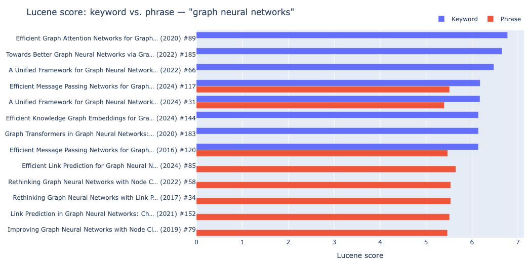
Figure 1. Keyword vs. Phrase Search.

The result is worth reading carefully. In this dataset, every paper in the Graph Neural Networks field contains the exact phrase, because the field name appears in its title and abstract. So both queries match essentially the same papers and their scores are close: 6.1 to 6.8 for keywords and 5.4 to 5.65 for the phrase.

What changes is which papers make the top eight. Only three of the eight appear in both lists, and the top result differs: keyword search ranks "Efficient Graph Attention Networks for Graph Neural Networks" first (6.774), while phrase search ranks "Efficient Link Prediction for Graph Neural Networks" first (5.649).

A plausible reason is that keyword scoring rewards papers that repeat the individual words, such as "graph" and "networks" in a title that also mentions graph attention networks, while phrase scoring only counts the phrase itself. Raw scores aren't directly comparable across the two query forms, so membership and order are the things to compare.

On noisier text, where the words in a query don't usually sit together, the phrase search would also drop papers entirely, which is the more familiar reason to use it.

Fuzzy Search

Appending ~ to a term enables Lucene's fuzzy matching, which finds terms within a given edit distance. A misspelled query like tranformer~ correctly matches transformer:

search_papers("tranformer~", top_k=3)

Example output:

Efficient Transformer Models for Natural Language Processing
Natural Language Processing | Transactions on Machine Learning and Data Mining | 2020 | Citations: 196
Score: 3.015
...

Without the ~, the misspelled query returns nothing. With it, Lucene finds the closest matching terms and scores them. This is useful for any field where exact spelling can't be guaranteed, such as technical terms or partially remembered titles.

Filtered Search

We can combine the full-text index with filters on structured node properties. There is one thing to be aware of: for full-text indexes, SEARCH doesn't allow a WHERE inside the clause. Filtering is a second step. The index first returns its top-scoring candidates, then a WHERE after it filters them by field, year or citation count:

MATCH (p)
SEARCH p IN (
    FULLTEXT INDEX paper_fulltext
    FOR $search_query
    LIMIT 200
)
SCORE AS score
WITH p, score
WHERE p.field = $field
  AND p.year >= $min_year
  AND p.citation_count >= $min_citations
RETURN p.title, p.field, p.venue, p.year, p.citation_count, score
ORDER BY score DESC
LIMIT $top_k

The two limits do different jobs. The LIMIT 200 inside SEARCH sets the size of the candidate pool, here every paper in the collection, and the final LIMIT $top_k trims the filtered results. If we asked the index for only the top five and filtered afterward, a selective filter could leave us with nothing. On a large collection, we would choose a pool big enough for our filters to leave enough results, without asking the index to score everything.

These are the same three filtered queries used in the Weaviate chapter. Weaviate ran them as hybrid searches, combining vectors and keywords, whereas this is keyword-only BM25, so we should expect overlap in the results rather than identical rankings:

# NLP papers from 2020 onwards with at least 100 citations
search_papers_filtered(
    "attention mechanisms and transformer architectures",
    field         = "Natural Language Processing",
    min_year      = 2020,
    min_citations = 100,
)

# Recent computer vision papers
search_papers_filtered(
    "object detection in real time",
    field    = "Computer Vision",
    min_year = 2022,
)

# Highly cited papers across all fields
search_papers_filtered(
    "self-supervised learning for representation learning",
    min_citations = 200,
)

The first query returns two papers (scores 3.350 and 3.154) and the second returns one (7.250). The third returns five: the three self-supervised learning papers score between 10.273 and 9.537, then the scores drop to 3.543 for the fourth paper, which matches only more generic terms such as "learning". With the default analyzer, an earlier run of the first query also returned papers scoring below 0.1, apparently matching only on common words such as "and". With stop words removed, that tail no longer appears.

Search Then Traverse: The Graph Layer

Full-text search answers "Which documents match?" Graph traversal answers "What is connected to those matches?" This section is where the two work together. We'll use the Lucene results as an entry point into the graph, then traverse CITES and AUTHORED relationships to discover related content. The pattern is always the same: SEARCH finds the initial set, then Cypher traverses from there.

In a synthetic graph, some papers have few connections, so the notebook runs ten candidate queries and measures each top result's neighborhood: how many papers it cites, how many cite it, and how strongly it is co-cited with others. It picks the richest as the demonstration query. That query is "protein structure prediction", whose top result, "Efficient Protein Structure Prediction for Bioinformatics" (score 12.926), cites 3 papers and is cited by 17.

What Does a Top Result Cite?

Starting from the highest-scoring paper, we'll follow outgoing CITES edges to see what it builds on. Note that citation_count is a property generated independently for each paper — it isn't derived from the CITES relationships in this graph. We use it here as a proxy for importance when ordering results.

MATCH (p)
SEARCH p IN (
    FULLTEXT INDEX paper_fulltext
    FOR $search_query
    LIMIT 1
)
SCORE AS score
WITH p, score
MATCH (p)-[:CITES]->(cited:Paper)
RETURN p.title AS source_title, score AS source_score,
       cited.title, cited.field, cited.year, cited.citation_count
ORDER BY cited.citation_count DESC
LIMIT $top_k

Example output:

Drug Discovery for Bioinformatics: A Scalable Approach
Bioinformatics | 2016 | Citations: 483

Improving Bioinformatics with Drug Discovery
Bioinformatics | 2016 | Citations: 467

Cryptographic Protocols in Cybersecurity: Challenges and Opportunities
Cybersecurity | 2016 | Citations: 283

What Cites a Top Result?

Traversing in the opposite direction — incoming CITES edges — finds papers that build on a highly relevant result:

MATCH (p)
SEARCH p IN (
    FULLTEXT INDEX paper_fulltext
    FOR $search_query
    LIMIT 1
)
SCORE AS score
WITH p, score
MATCH (citing:Paper)-[:CITES]->(p)
RETURN p.title AS source_title, score AS source_score,
       citing.title, citing.field, citing.year, citing.citation_count
ORDER BY citing.year DESC
LIMIT $top_k

The most recent citing papers include "A Unified Framework for Reinforcement Learning using Hierarchical Rl" (2024), "Efficient Malware Classification for Cybersecurity" (2024), and "Meta-Learning for Machine Learning: A Scalable Approach" (2024). Citations reach across fields because the generator only biases them toward related fields; it doesn't confine them.

Visualizing the Citation Network

We can visualize the citation neighborhood of the top result as an interactive graph with neo4j-viz. In Figure 2, the central red node is the top-scoring paper, blue nodes are papers it cites, and green nodes are papers that cite it. Arrows point from the citing paper to the cited paper, and node size reflects citation count. In the notebook, hovering over a node shows the full title, year, and citation count.

# One Cypher query returns the top result with the papers it cites and the papers that cite it
nodes, relationships = {}, []

nodes[top["id"]] = Node(id=top["id"], caption=short(top["title"]),
                        properties={"role": "Top result", "citations": top["citations"]})
for p in top["cited"]:
    nodes[p["id"]] = Node(id=p["id"], caption=short(p["title"]),
                          properties={"role": "Cites", "citations": p["citations"]})
    relationships.append(Relationship(source=top["id"], target=p["id"]))
for p in top["citing"]:
    nodes[p["id"]] = Node(id=p["id"], caption=short(p["title"]),
                          properties={"role": "Cited by", "citations": p["citations"]})
    relationships.append(Relationship(source=p["id"], target=top["id"]))

VG = VisualizationGraph(nodes=list(nodes.values()), relationships=relationships)
VG.color_nodes(property="role", colors={
    "Top result": "#EF553B", "Cites": "#636EFA", "Cited by": "#00CC96"})
VG.resize_nodes(property="citations", node_radius_min_max=(14, 40))
VG.render(height="520px")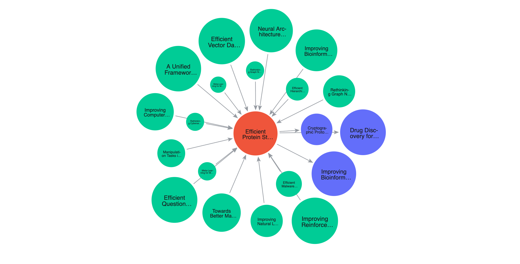

Figure 2. Citation Network.

This kind of neighborhood visualization isn't something we'd get from a search engine, as it requires the graph.

Find Other Work by the Same Authors

From the top result, we'll traverse AUTHORED edges to the authors, then follow their other AUTHORED edges to find their other papers:

MATCH (p)
SEARCH p IN (
    FULLTEXT INDEX paper_fulltext
    FOR $search_query
    LIMIT 1
)
SCORE AS score
WITH p, score
MATCH (a:Author)-[:AUTHORED]->(p)
MATCH (a)-[:AUTHORED]->(other:Paper)
WHERE other <> p
RETURN p.title AS source_title, score AS source_score,
       a.name AS author, other.title, other.field, other.year,
       other.citation_count
ORDER BY other.citation_count DESC
LIMIT $top_k

The highest-cited results are papers by Chen Singh and Lena Li, two of the authors of the top result, including "Improving Computer Vision with Generative Adversarial Networks" (475 citations) and "Efficient Multi-Agent Systems for Reinforcement Learning" (433). This is the kind of discovery path that's natural in a graph but would typically require additional application-side queries or data modeling outside the search index.

Co-Citation Discovery

Two papers are co-cited when a third paper cites both of them. Frequently co-cited papers can indicate related research topics, shared foundations, or intellectual proximity — a relationship that doesn't appear in the papers themselves, only in how others use them:

MATCH (p)
SEARCH p IN (
    FULLTEXT INDEX paper_fulltext
    FOR $search_query
    LIMIT 1
)
SCORE AS score
WITH p, score
MATCH (citing:Paper)-[:CITES]->(p)
MATCH (citing)-[:CITES]->(cocited:Paper)
WHERE cocited <> p
WITH p, score, cocited, count(citing) AS shared_citations
RETURN p.title AS source_title, score AS source_score,
       cocited.title, cocited.field, cocited.year, shared_citations
ORDER BY shared_citations DESC
LIMIT $top_k

For our top result, the most co-cited paper is "Drug Discovery for Bioinformatics: A Scalable Approach" with 6 shared citing papers, followed by "Rethinking Robotics with Imitation Learning" with 5, and three papers with 4 each. The Robotics paper is a reminder that the generator's field bias is only a bias. Co-citation analysis is a classical technique in bibliometrics, and here it is a single Cypher query.

Traversing From More Than One Result

So far we've started from the single best hit. The same pattern works from the top N results, and aggregation then surfaces something no single result shows: the papers that several of the best matches have in common. Here we ask which papers are cited by the most of the top five results, a rough proxy for foundational work on the topic:

MATCH (p)
SEARCH p IN (
    FULLTEXT INDEX paper_fulltext
    FOR $search_query
    LIMIT 5
)
SCORE AS score
WITH p, score
MATCH (p)-[:CITES]->(ref:Paper)
RETURN ref.title AS title, ref.field AS field, ref.year AS year,
       ref.citation_count AS citations,
       count(DISTINCT p) AS cited_by_hits
ORDER BY cited_by_hits DESC, citations DESC
LIMIT $top_k

Two papers, "Drug Discovery for Bioinformatics: A Scalable Approach" and "Improving Bioinformatics with Drug Discovery," are each cited by two of the five best matches, ahead of papers cited by only one. A standalone search engine would return the five matches and stop there.

When to Use This

Neo4j's full-text search is worth reaching for when our data are already in a graph, and we want to add keyword search without operating a separate service. The setup is minimal: one Cypher command creates the index, one clause queries it, and we immediately get phrase matching, fuzzy matching, field boosting, and BM25 relevance scoring. Because the index is updated in the same transaction as the data, there is no synchronization pipeline to build or monitor.

The search-then-traverse pattern is the real differentiator. If our data have relationships, such as citations, authorship, product categories, or social connections, and we want search to serve as an entry point into those relationships, Neo4j gives us both in one place.

It is not the right choice for every workload. A dedicated search engine offers capabilities that weren't part of what we used here, such as faceted aggregations and result highlighting, and it lets us scale search independently of the database. If search traffic is large, if it needs different hardware from the graph workload, or if the data have no meaningful relationships, a separate service may be the better fit. The SEARCH behavior described above also matters at scale: the index returns a bounded candidate set, and filters apply afterward, so queries with very selective filters need a candidate pool sized for them.

For purely semantic workloads where we want vector similarity rather than keyword matching, Neo4j also supports vector indexes, which we can combine with full-text search in the same query. But for the common case where keyword search and graph traversal belong together, the built-in Lucene integration is often all we need.

Summary

We've seen how to create a multi-property full-text index in Neo4j, query it with the SEARCH clause using keyword, phrase, and fuzzy search, escape user input and boost fields, combine the results with structured property filters, and use them as the entry point for graph traversals that follow citations, authorship, co-citation, and multiple matches at once.

Further examples of Neo4j's multi-model capabilities can be found in the free online book Neo4j Beyond the Graph.

The full source code is available on GitHub.