Master Production-Ready Big Data, Apache Spark Jobs in Databricks and Beyond: An Expert Guide
Refine Apache Spark performance in Databricks with strategies. Includes expert insights, PySpark examples, and diagrams for efficient data processing.
Join the DZone community and get the full member experience.
Join For FreeThis iteration is based on existing experience scaling big data with Apache Spark workloads and uses more refinements by still preserving the eight most important strategies but moving high-value but less important strategies — such as preferring narrow transformations, applying code-level best practices, leveraging Databricks Runtime features, and optimizing cluster configuration — to a Miscellaneous section, thereby not losing focus on impactful areas such as shuffles and memory, but still addressing them thoroughly.
Diagrams for in-phased insights and example code can be completely executed in Databricks or vanilla Spark sessions, and for all of these to be worth your time, the application will yield unbelievable performance benefits, often in the range of 5–20x in real-world pipelines.
Optimization Strategies
1. Partitioning and Parallelism
Strategy: Use repartition() to enhance parallelism before shuffle-intensive operations like joins, and coalesce() to minimize partitions pre-write to prevent small-file issues that hammer storage metadata.
from pyspark.sql import SparkSession
from pyspark.sql.functions import rand

spark = SparkSession.builder.appName("PartitionExample").getOrCreate()

# Sample DataFrame creation
data = [(i, f"val_{i}") for i in range(1000000)]
df = spark.createDataFrame(data, ["id", "value"])

# Repartition for parallelism before a join or aggregation
df_repartitioned = df.repartition(200, "id")  # Shuffle to 200 even partitions

# Perform a sample operation (e.g., groupBy)
aggregated = df_repartitioned.groupBy("id").count()

# Coalesce before writing to reduce output files
aggregated_coalesced = aggregated.coalesce(10)
aggregated_coalesced.write.mode("overwrite").parquet("/tmp/output")

print(f"Partitions after repartition: {df_repartitioned.rdd.getNumPartitions()}")
print(f"Partitions after coalesce: {aggregated_coalesced.rdd.getNumPartitions()}")Explanation: Partitioning is foundational for parallelism of tasks and load balancing in Spark's distributed model. repartition(n) ensures even data spread via full shuffle, ideal pre-joins to avoid executor overload. coalesce(m) (where m < current partitions) merges locally for efficient writes, cutting I/O costs in Databricks' Delta or S3.
Risks: Over-repartitioning increases shuffle overhead; monitor via Spark UI's "Input Size" metrics. Benefits: Scalable for TB-scale data; universal across Spark envs.
Diagram: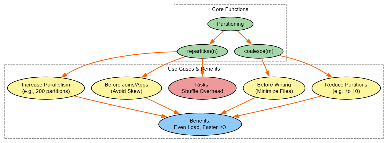
2. Caching and Persistence
Strategy: Cache or persist reusable DataFrames to skip recomputation in iterative or multi-use scenarios.
from pyspark.sql import SparkSession
from pyspark.storagelevel import StorageLevel

spark = SparkSession.builder.appName("CachingExample").getOrCreate()

# Create a sample DataFrame
df = spark.range(1000000).withColumn("squared", spark.range(1000000).id ** 2)

# Cache for memory-only (default)
df.cache()
print("First computation (uncached effectively, but sets cache):", df.count())

# Reuse: Faster second time
print("Second computation (from cache):", df.count())

# Persist with custom level (e.g., memory and disk)
df.persist(StorageLevel.MEMORY_AND_DISK)
print("Persisted count:", df.count())

# Clean up
df.unpersist()Explanation: Recomputation kills performance in loops or DAG branches. cache() uses MEMORY_ONLY; persist() allows levels like MEMORY_AND_DISK for spill resilience. In Databricks, this leverages fast NVMe; watch memory usage to avoid evictions.
Benefits: Up to 10x speedup in ML training.
Risks: Memory exhaustion – use spark.ui to track.
Diagram: 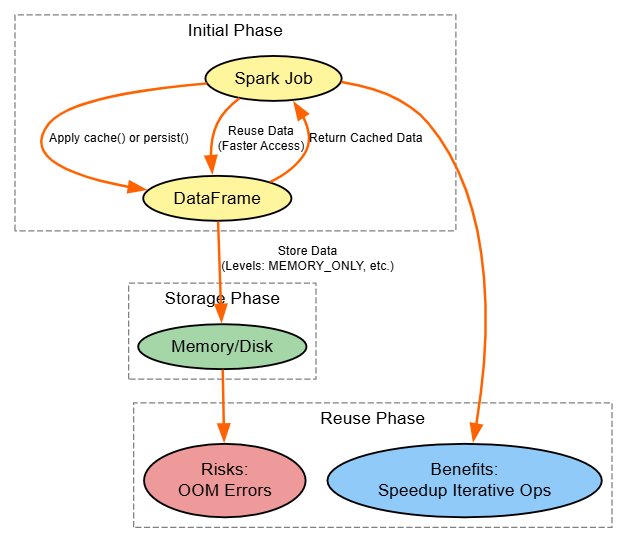
3. Predicate Pushdown
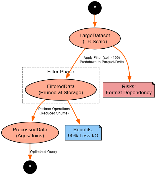
Strategy: Filter early to leverage storage-level pruning, especially with Parquet/Delta.
from pyspark.sql import SparkSession
from pyspark.sql.functions import col

spark = SparkSession.builder.appName("PushdownExample").getOrCreate()

# Read from Parquet (supports pushdown)
df = spark.read.parquet("/tmp/large_dataset.parquet")  # Assume pre-written large file

# Early filter: Pushed down to storage
filtered_df = df.filter(col("value") > 100).filter(col("category") == "A")

# Further ops: Less data shuffled
result = filtered_df.groupBy("category").sum("value")
result.show()

# Compare explain plans
df.explain()  # Without filter
filtered_df.explain() # With pushdown visibleExplanation: Pushdown skips irrelevant data at the source, slashing reads. Delta Lake enhances with stats; universal but format-dependent (Parquet, yes; JSON, no).
Benefits: Network savings.
Risks: Over-filtering hides data issues.
Diagram:
4. Skew Handling
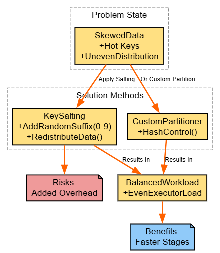
Strategy: Salt keys or custom-partition to even out distributions.
from pyspark.sql import SparkSession
from pyspark.sql.functions import col, concat, lit, rand, floor

spark = SparkSession.builder.appName("SkewExample").getOrCreate()

# Skewed DataFrame
skewed_df = spark.createDataFrame([(i % 10, i) for i in range(1000000)], ["key", "value"])  # Many duplicates on low keys

# Salt keys: Append random suffix (0-9)
salted_df = skewed_df.withColumn("salted_key", concat(col("key"), lit("_"), floor(rand() * 10).cast("string")))

# Group on salted key, then aggregate
temp_agg = salted_df.groupBy("salted_key").sum("value")
# Remove salt for final result
final_agg = temp_agg.withColumn("original_key", col("salted_key").substr(1, 1)).groupBy("original_key").sum("sum(value)")

final_agg.show()Explanation: Skew starves executors; salting disperses hot keys temporarily. Custom partitioners (via RDDs) offer precision. Check UI task times.
Benefits: Balanced execution.
Risks: Extra compute for salting.
Diagram:
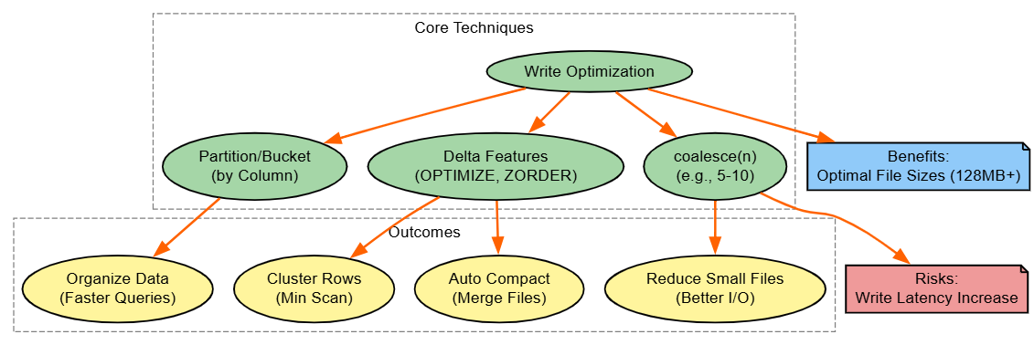
5. Optimize Write Operations
Strategy: Bucket/partition wisely, coalesce files, use Delta's Optimize/Z-Order.
from pyspark.sql import SparkSession

spark = SparkSession.builder.appName("WriteOptExample").getOrCreate()

# Sample DataFrame
df = spark.range(1000000).withColumn("category", (spark.range(1000000).id % 10).cast("string"))

# Partition by column for query efficiency
df.write.mode("overwrite").partitionBy("category").parquet("/tmp/partitioned")

# For Delta: Write, then optimize
df.write.format("delta").mode("overwrite").save("/tmp/delta_table")
spark.sql("OPTIMIZE delta.`/tmp/delta_table` ZORDER BY (id)")

# Coalesce before write
df.coalesce(5).write.mode("overwrite").parquet("/tmp/coalesced")Explanation: Writes create file explosions; coalescing consolidates. Delta's Z-Order clusters for scans;
Benefits: Faster reads; Databricks-specific but portable via Hive.
Diagram:
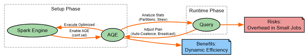
6. Leverage Adaptive Query Execution (AQE)
Strategy: Enable AQE for runtime tweaks like auto-skew handling.
from pyspark.sql import SparkSession

spark = SparkSession.builder.appName("AQEExample").getOrCreate()

# Enable AQE
spark.conf.set("spark.sql.adaptive.enabled", "true")
spark.conf.set("spark.sql.adaptive.coalescePartitions.enabled", "true")

# Sample join that benefits from AQE (auto-broadcast if small)
large_df = spark.range(1000000)
small_df = spark.range(100)
result = large_df.join(small_df, large_df.id == small_df.id)

result.explain()  # Shows adaptive plans
result.show()Explanation: AQE adjusts post-stats (e.g., reduces partitions); benefits: Hands-off optimization; Spark 3+ universal.
Diagram:
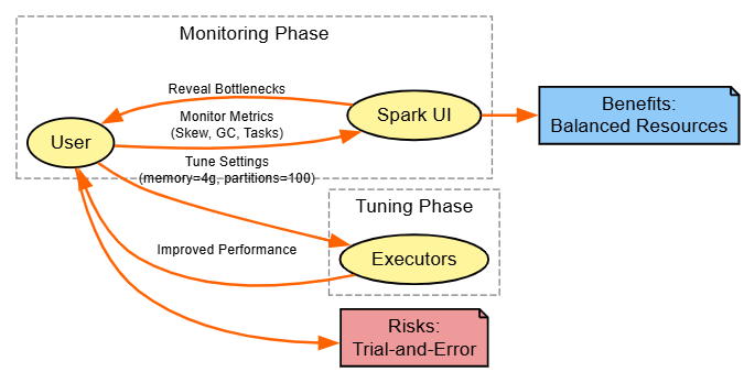
7. Job and Stage Optimization
Strategy: Tune via Spark UI insights, adjusting memory/parallelism.
from pyspark.sql import SparkSession

spark = SparkSession.builder.appName("TuneExample") \
    .config("spark.executor.memory", "4g") \
    .config("spark.sql.shuffle.partitions", "100") \
    .getOrCreate()

# Sample job
df = spark.range(10000000).groupBy("id").count()
df.write.mode("overwrite").parquet("/tmp/tuned")

# After run, check UI for GC/stages; adjust configs iterativelyExplanation: UI flags GC (>10% bad); tune shuffle.partitions to match cores.
Benefits: Resource efficiency; universal.
Diagram:
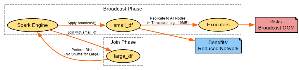
8. Optimize Joins With Broadcast Hash Join (BHJ)
Strategy: Broadcast small sides to eliminate shuffles.
from pyspark.sql import SparkSession
from pyspark.sql.functions import broadcast

spark = SparkSession.builder.appName("BHJExample").getOrCreate()

# Large and small DataFrames
large_df = spark.range(1000000).toDF("key")
small_df = spark.range(100).toDF("key")

# Broadcast small for BHJ
result = large_df.join(broadcast(small_df), "key")
result.explain()  # Shows BroadcastHashJoin
result.show()Explanation: BHJ copies small DF to nodes; tune spark.sql.autoBroadcastJoinThreshold.
Benefits: Shuffle-free.
Risks: Memory for broadcast.
Diagram:
Miscellaneous Strategies
These additional techniques complement the core set, offering targeted enhancements for specific scenarios. While not always foundational, they can provide significant boosts in code efficiency, platform-specific acceleration, and infrastructure tuning.
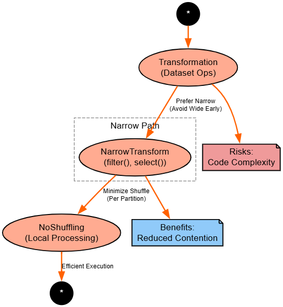
Prefer Narrow Transformations
Strategy: Favor narrow transformations like filter() and select() over wide ones like groupBy() or join().
from pyspark.sql import SparkSession
from pyspark.sql.functions import col

spark = SparkSession.builder.appName("NarrowExample").getOrCreate()

# Sample large DataFrame
df = spark.range(1000000).withColumn("value", spark.range(1000000).id * 2)

# Narrow: Filter and select first (no shuffle)
narrow_df = df.filter(col("value") > 500000).select("id")

# Then wide: GroupBy (shuffle only on reduced data)
result = narrow_df.groupBy("id").count()
result.show()Explanation: Narrow ops process per-partition, avoiding shuffles; chain them early to prune. Benefits: Lower overhead
Risks: Over-chaining increases complexity in code.
Diagram:
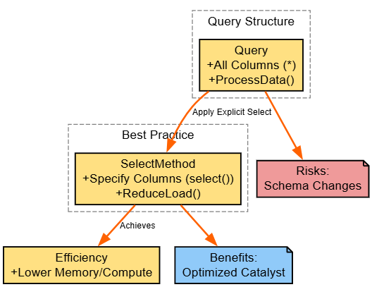
Code-Level Best Practices
Strategy: Use select() to specify columns explicitly, avoiding *.
from pyspark.sql import SparkSession

spark = SparkSession.builder.appName("CodeBestExample").getOrCreate()

# Sample wide table
df = spark.createDataFrame([(1, "A", 100, "extra1"), (2, "B", 200, "extra2")], ["id", "category", "value", "unused"])

# Bad: Select all (*)
all_df = df.select("*")  # Loads unnecessary columns

# Good: Select specific
slim_df = df.select("id", "category", "value")

# Process: Less memory used
result = slim_df.filter(col("value") > 150)
result.show()Explanation: * loads extras, increasing memory; select() trims.
Benefits: Leaner pipelines; risks: Missing columns in evolving schemas.
Diagram:
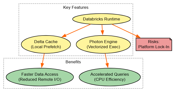
Utilize Databricks Runtime Features
Strategy: Harness Delta Cache and Photon for I/O and compute acceleration.
Code
from pyspark.sql import SparkSession

spark = SparkSession.builder.appName("RuntimeFeaturesExample").getOrCreate()

# Assume Databricks Runtime with Photon enabled
spark.conf.set("spark.databricks.delta.cache.enabled", "true")  # Delta Cache

# Read Delta (caches automatically)
df = spark.read.format("delta").load("/tmp/delta_table")

# Query: Benefits from cache/Photon vectorization
result = df.filter(col("value") > 100).groupBy("category").sum("value")
result.show()Explanation: Delta Cache preloads locally; Photon vectorizes.
Benefits: Latency drops; Databricks-only, emulate with manual caching elsewhere.
Diagram
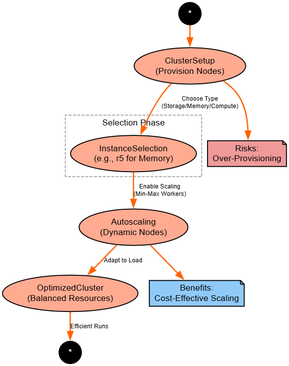
Optimize Cluster Configuration for Big Data
Strategy: Select instance types and enable autoscaling. For example, AWS EMR, etc.
# This is configured via Databricks UI/CLI, not code, but example job config:
# In Databricks notebook or job setup:
# Cluster: Autoscaling enabled, min 2-max 10 workers
# Instance: i3.xlarge (storage-optimized) or r5.2xlarge (memory-optimized)

from pyspark.sql import SparkSession

spark = SparkSession.builder.appName("ClusterOptExample").getOrCreate()

# Run heavy job: Autoscaling handles load
df = spark.range(100000000).groupBy("id").count()  # Scales up automatically
df.show()Explanation: Match instances to workload (e.g., memory for joins); autoscaling adapts.
Benefits: Cost savings; Databricks-specific, but can be applied to AWS EMR, etc., with auto- and managed-scaling of instance configuration JSON during cluster bootstrap.
Diagram
Applicability to Databricks and Other Spark Environments
- Universal: Some of these methods apply to EMR, Synapse, and other Spark platforms, like Partitioning, caching, predicate pushdown, skew handling techniques, narrow transformations, coding practices, AQE, job optimization, and BHJ.
- Databricks-specific: Write operations with Delta, features in the Runtime, cluster configuration (and configuration changes) are all native to Databricks (but can be leveraged with alternatives like Iceberg or some manual tuning).
Conclusion
In this article, I tried to demonstrate eight core strategies that underpin addressing shuffle, memory, and I/O bottlenecks, and improving efficiency. The miscellaneous section describes some subtle refinement approaches, platform-specific improvements, and infrastructure tuning. You now have flexibility and variability in workloads, including ad hoc queries and production ETL pipelines. Collectively, these 12 strategies (core and misc.) promote a way of thinking holistically about optimization. Start by profiling in Spark UI, adaptively implement incremental improvements using the snippets provided here, and benchmark exhaustively to demonstrate the improvements (using metrics for each). By applying these techniques in Databricks, you will not only reduce costs and latency but also build scalable, resilient big data engineering solutions.
As Spark development (2025 trends) continues to expand, please revisit this reference and new tools, such as MLflow, for experimentation capabilities, moving bottlenecks into breakthroughs.
Opinions expressed by DZone contributors are their own.
Comments