Machine Learning for CI/CD: Predicting Deployment Durations and Improving DevOps Agility

The speed and reliability of CI/CD pipelines directly impact developer velocity and release quality. However, deployment durations can vary widely due to factors like code complexity, pipeline structure, testing strategies, and environment configurations. This article explores how to build a machine learning regression model that predicts deployment time based on features derived from CI/CD metadata, code metrics, and infrastructure events.

Why Predict Deployment Duration?

Predicting deployment time can:

• Improve release planning and scheduling
• Identify delays and pipeline bottlenecks in advance
• Set realistic deployment expectations for teams
• Assist in SLA monitoring for critical deployments
• Optimize CI/CD configurations to reduce waste

A custom ML solution provides greater insights than static benchmarking by learning from actual deployment history.

Key CI/CD Data Features for Modeling

Feature Categories:

Pipeline Metadata

pipeline_id, stage_name, execution_env, trigger_type

Code Attributes

files_changed, lines_added, lines_removed, test_coverage, codebase_size

Infrastructure Metrics

runner_type, resource_class, num_parallel_jobs, artiface_size, container_boot_time

Temporal Indicators

hour_of_day, day_of_week, is_weekend, deploy_window

Historical Signals

avg_duration_by_branch, previous_duration, rolling_mean_duration

Hotfix-related Features

branch_type (e.g., feature, hotfix, release)

commit_message_keywords (e.g., contains 'fix' or 'incident')

incident_flag (derived from incident logs or tagging)

Tool/Stage Change Features

stage_count, stage_names, new_tool_flag, tool_type

introduced_tool_duration_estimate (e.g., historical tool execution time)

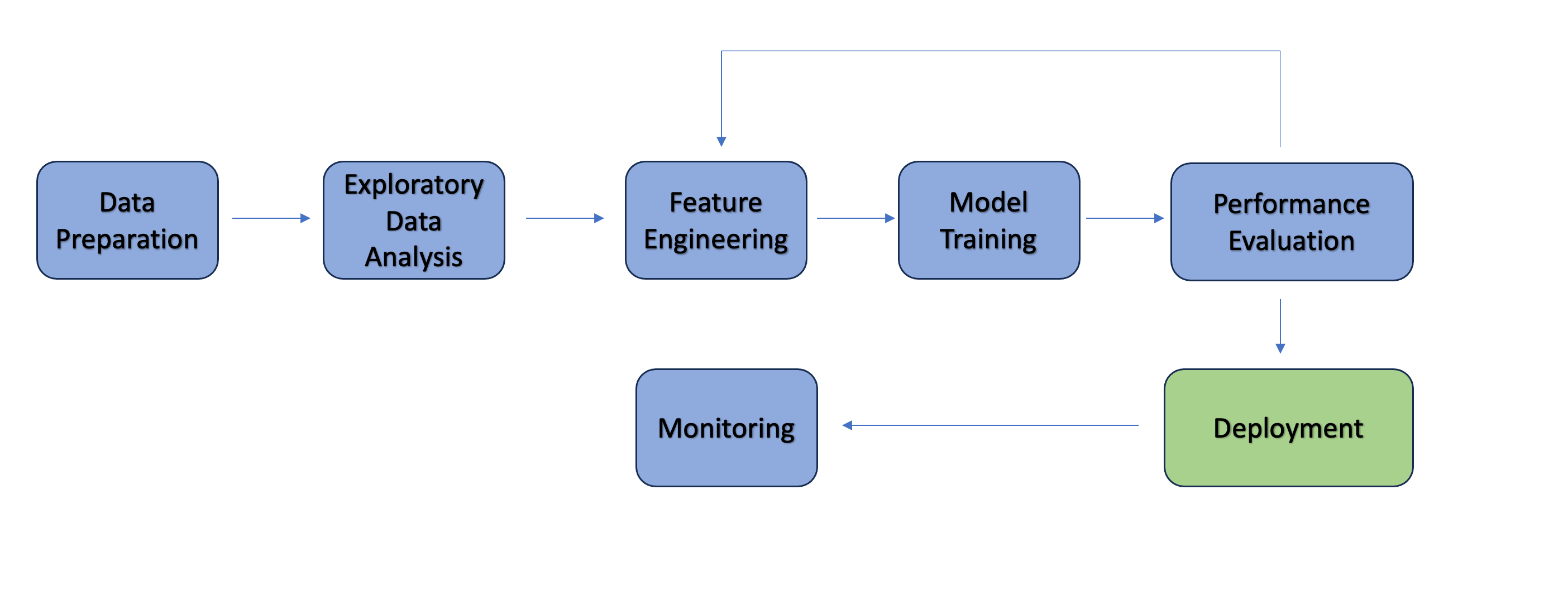
ML Regression Workflow

To build a robust and interpretable deployment duration prediction model, we follow a detailed ML workflow that includes univariate and multivariate analysis, handling outliers, correcting skewness, detecting multicollinearity, validation, and deployment. Each step plays a critical role in ensuring model quality and trustworthiness.

Before diving into the steps, let’s briefly explore the regression algorithms considered for this use case and the rationale behind choosing them:

Choosing the Right Regression Model

Several regression models were tested:

• Linear Regression: Simple, interpretable, but struggles with non-linear patterns common in CI/CD durations.
• Random Forest Regressor: Great for capturing non-linearities, but can be heavy on resources and less granular in prediction tuning.
• XGBoost Regressor: Performs well with tabular data, handles skew, highlights feature importance, and supports fast training. It also works effectively with log-transformed targets.

For this article, we used XGBoost because it offered the best tradeoff between performance, interpretability, and speed.

1. Data Ingestion and Initial Processing

To begin, ingest historical CI/CD data and convert the relevant timestamp fields to enable extraction of hour and weekday features. These temporal elements help capture predictable patterns, such as longer queues on weekday mornings.

import pandas as pd
ci_logs = pd.read_csv("ci_cd_logs.csv")
ci_logs['timestamp'] = pd.to_datetime(ci_logs['timestamp'])
ci_logs['hour'] = ci_logs['timestamp'].dt.hour
ci_logs['weekday'] = ci_logs['timestamp'].dt.dayofweek

2. Univariate and Multivariate Analysis

Before modeling, explore each feature to understand its distribution and relationships:

Univariate Analysis: Use histograms and box plots to check distributions of numerical features like files_changed, artifact_size_mb, and deployment_duration_sec.

import seaborn as sns
import matplotlib.pyplot as plt
sns.histplot(ci_logs['deployment_duration_sec'], bins=30)
plt.title("Deployment Duration Distribution")
plt.show()

Multivariate Analysis: Use correlation heatmaps and pair, scatter plots to evaluate feature relationships.

sns.heatmap(ci_logs.corr(), annot=True, fmt=".2f")
plt.title("Feature Correlation Heatmap")
plt.show()

Obvious Multivariate Patterns to Explore

• Lines of Code Change vs Execution Time: Larger code diffs (high code_change_intensity) tend to increase deployment durations due to more build/test activity.
• Peak Hours vs Deployment Time: Deployments triggered during peak hours (e.g., 9 AM – 12 PM) may experience queue delays.
• Weekend Deployments: is_weekend = True often leads to faster deployments due to lower pipeline contention.
• Artifact Density vs Deployment Time: A higher ratio of artifact size to file count (artifact_density)  may indicate compressed or packaged assets, potentially slowing down deployment steps.
• Parallel Jobs vs Duration: When available, analyze num_parallel_jobs to see if more concurrency leads to time savings or overhead from orchestration.

3. Data Quality Checks

Before training a model, it’s crucial to ensure your dataset is clean and consistent:

• Check for missing values:

print(ci_logs.isnull().sum())

• Drop records with missing target or key features:

ci_logs.dropna(subset=['deployment_duration_sec', 'files_changed'], inplace=True)

• Remove duplicate logs if any:

ci_logs.drop_duplicates(inplace=True)

4. Handling Missing and Skewed Data

Some numeric fields might have sparse missing values. We can fill them using median imputation. Additionally, deployment durations are often right-skewed, so log transformation helps normalize the distribution:

ci_logs['artifact_size_mb'].fillna(ci_logs['artifact_size_mb'].median(), inplace=True)
import numpy as np
ci_logs['log_duration'] = np.log1p(ci_logs['deployment_duration_sec'])

5. Outlier Detection and Removal

Outliers can distort regression models. Use interquartile range (IQR) to remove unusually fast or slow deployments:

Q1 = ci_logs['deployment_duration_sec'].quantile(0.25)
Q3 = ci_logs['deployment_duration_sec'].quantile(0.75)
IQR = Q3 - Q1
ci_logs = ci_logs[(ci_logs['deployment_duration_sec'] >= Q1 - 1.5*IQR) & 
                  (ci_logs['deployment_duration_sec'] <= Q3 + 1.5*IQR)]

6. Feature Engineering

Generate new, domain-specific features:

•  is_weekend helps distinguish slow weekend deployments
•  code_change_intensity sums total code delta
•  artifact_density normalizes artifact size per file

7. Train/Test Split

Split the data for training and validation. We predict log_duration instead of raw duration for better stability.

from sklearn.model_selection import train_test_split
features = ['files_changed', 'code_change_intensity', 'hour', 'is_weekend', 'artifact_density']
X = ci_logs[features]
y = ci_logs['log_duration']
X_train, X_test, y_train, y_test = train_test_split(X, y, test_size=0.3)

Using 70/30 split to divide the dataset into training and testing subsets:

• 70% (Training Set): Used to learn the patterns.
• 30% (Test Set): Held out to evaluate generalization performance.

This ensures a balanced split for validation while retaining enough samples for model learning.

8. Model Training (XGBoost)

Train a boosted tree model which handles non-linear interactions and feature importance effectively.

from xgboost import XGBRegressor
model = XGBRegressor(objective='reg:squarederror', n_estimators=100, learning_rate=0.1)
model.fit(X_train, y_train)

9. Model Validation and Evaluation

Use multiple metrics to evaluate performance on the test set and assess generalization. Evaluate the model using standard regression metrics and inverse-transform the log predictions.

from sklearn.metrics import mean_absolute_error, mean_squared_error, r2_score

y_pred_log = model.predict(X_test)
y_pred = np.expm1(y_pred_log)
y_true = np.expm1(y_test)

mae = mean_absolute_error(y_true, y_pred)
rmse = np.sqrt(mean_squared_error(y_true, y_pred))
r2 = r2_score(y_true, y_pred)

print("MAE:", mae)
print("RMSE:", rmse)
print("R^2 Score:", r2)

Results Example:

• MAE: 48.2 seconds — on average, predictions are within 1 minute
• RMSE: 60.3 seconds — measures average error magnitude
• R² Score: 0.85 — strong model fit

Use Cases in Real Time

Shift-Left Strategy Enablement

Shift-left practices encourage teams to catch defects and performance issues early in the development lifecycle. A deployment duration prediction model aligns perfectly with this philosophy:

• Proactive performance awareness: Developers receive immediate feedback on how changes might impact deployment time—before merging code.
• Faster experimentation: By forecasting the overhead introduced by additional tests or build steps, teams can make smarter decisions about when and where to run them.
• Guardrail policies: Integrate duration thresholds into pre-merge CI checks to prevent unusually long or risky jobs from merging into main branches.
• Branch optimization: Teams can analyze and restructure their pipeline stages for more efficient execution based on predicted duration patterns.

Example: A developer adds a new stage to verify database schema migrations. If the ML model predicts it adds 5+ minutes to deploy, they can explore optimization strategies or schedule it for nightly builds.

Introducing a New Tool or Stage in the CI/CD Pipeline

When a new tool (e.g., security scanner, code coverage reporter, container registry step) or an entirely new stage is introduced in the CI/CD workflow, it can introduce latency or unexpected side effects. Predicting deployment durations in advance helps mitigate the risks associated with these changes:

• Baseline comparison: ML models can forecast the expected increase in deployment duration after adding the new tool.
• Test impact pre-merge: Teams can simulate the effect of the new stage on real data before rolling it into the mainline pipeline.
• Automated rollout monitoring: If a new stage increases deployment time by >15%, alert teams or auto-revert the change.
• Prioritization of tasks: Use predictions to defer new tools to off-peak hours or specific branches.

Example: If adding a static analysis tool is predicted to add 2.5 minutes per deployment on average, it might be run only on staging or nightly builds initially.

Hotfix Acceleration with Deployment Time Prediction

In fast-moving production environments, teams often need to push hotfixes to resolve incidents quickly. However, long or unpredictable deployment durations can delay fixes and increase MTTR (mean time to resolution). By forecasting deployment times:

• Teams can prioritize fast paths: Knowing a hotfix from a stable branch will deploy in 90 seconds allows incident commanders to proceed confidently.
• Avoid bottlenecks: If the model predicts longer-than-average durations during peak hours (e.g., Mondays 9 AM), the team can switch runners or delay non-urgent builds.
• Trigger automated alerts: If the predicted deployment time exceeds a threshold, route the hotfix through a lighter CI profile.

Example: If the model predicts a 4-minute deploy for a 1-line hotfix, it could signal queue congestion or configuration drift.

Conclusion

By building a machine learning regression model for deployment forecasting, DevOps and platform teams can significantly improve observability, efficiency, and trust in CI/CD systems. The result is faster iteration, better team communication, and more intelligent infrastructure scaling.