Recursive Feature Elimination in Practice
Learn about Recursive Feature Elimination (RFE) to reduce feature count, boost accuracy, prevent overfitting, and build efficient machine learning models.
Join the DZone community and get the full member experience.
Join For FreeThe effectiveness of machine learning models often hinges on a deceptively simple question: Which features actually matter? The challenge becomes particularly evident as datasets grow larger and more complex. Modern data collection gives us access to hundreds or even thousands of features, but quantity doesn't always translate to quality. Processing all these features wastes computational resources and disrupts your model's performance.
Feature selection addresses this challenge by identifying the subset of features that contribute most meaningfully to your model's predictions. While several approaches exist for tackling this problem, Recursive Feature Elimination (RFE) stands out for its systematic and interpretable approach. By iteratively removing less important features, RFE helps you build models that are both more efficient and more accurate.
This guide will walk you through building a robust RFE system from scratch. Here’s what we’ll do:
- Reduce feature count while maintaining or improving model accuracy
- Identify feature importance with quantifiable metrics
- Validate selection stability through repeated testing
- Visualize feature elimination impact on model performance
But first things first, what exactly is RFE?
What Is RFE?
At its core, RFE is a feature selection method that works by recursively removing features and building a model with the remaining ones. By evaluating the model's performance at each step, RFE pinpoints the features that contribute the most to accurate predictions. A good analogy for this would be to think of it as a game of elimination where the least valuable features are eliminated one by one until only the most important ones remain.
For example, in a customer churn prediction model with 50 features, RFE might identify that just 15 features (such as payment history, usage patterns, and support tickets) capture 95% of the predictive power. So you’ll be able to remove the other 35 features without the accuracy taking a hit.
Now that we understand the basic concept of RFE, let's explore why it's become such a valuable tool in the machine learning toolbox.
Why Use RFE?
RFE offers several benefits:
- Improved model accuracy. By focusing on the most relevant features, RFE can help improve the accuracy of your machine learning model.
- Reduced overfitting. Removing less important features can prevent your model from learning noise in the data and overfitting to the training set.
- Faster training. With fewer features, your model will train faster.
- Enhanced interpretability. A simpler model with fewer features is easier to understand and interpret and will make it easier to explain your model's predictions.
Understanding these benefits helps explain RFE's popularity, but to truly make the best use of it, we need to dive into the mechanics of how it operates.
How Does It Work?
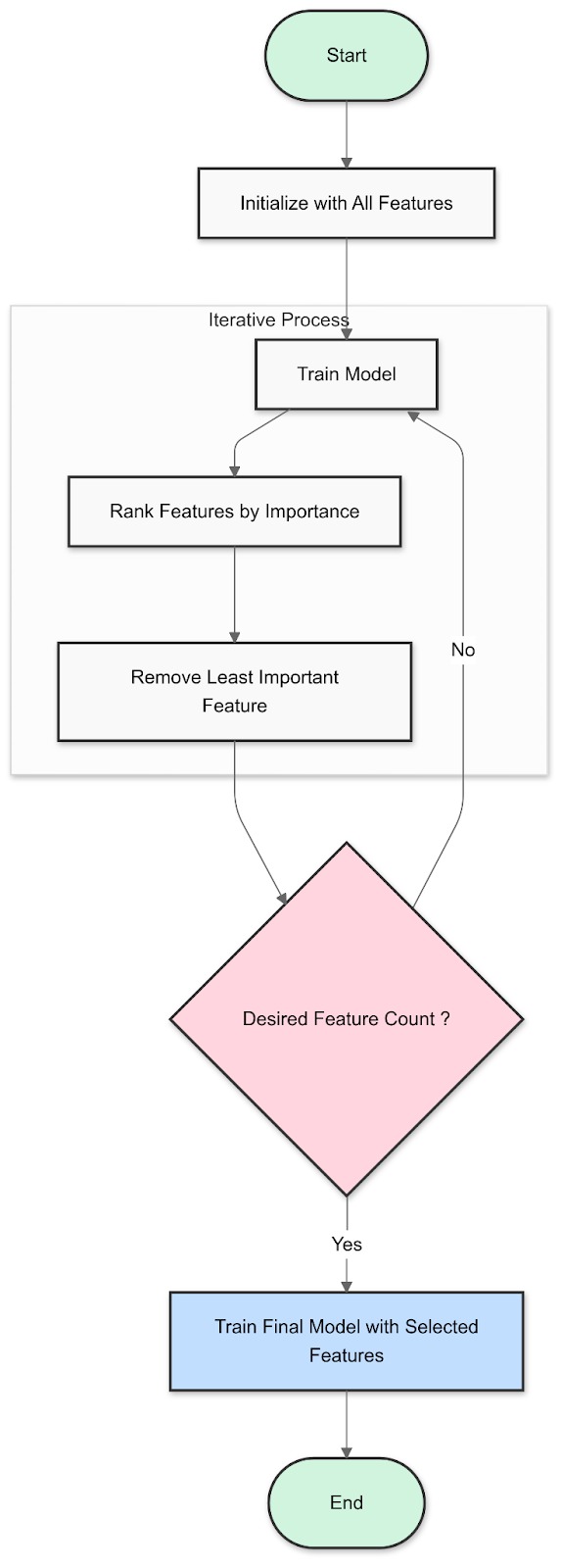
Fig 1: How Recursive Feature Elimination Works
- Train a model. Start by training your chosen machine learning model (e.g., a linear regression or a decision tree) using all the features in your dataset.
- Rank features. Determine the importance of each feature based on the model's coefficients or feature importances. This ranking tells you which features have the strongest relationship with the target variable.
- Eliminate the least important feature. Remove the feature with the lowest ranking from your dataset.
- Repeat. Retrain the model with the remaining features, rank them again, and eliminate the least important one. Repeat this process until you reach the desired number of features.
While this process might sound straightforward in theory, implementing it effectively requires careful attention to detail and proper coding practices. Let's walk through a complete implementation that you can adapt for your own projects.
Implementing RFE Step-by-Step
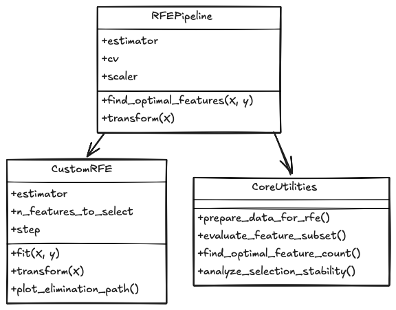
Below (refer to fig 2), you’ll see an overview of how we’ll implement the RFE process.
Now, let's dive into the practical implementation of RFE.
Before you run the above code on your system, make sure you have the following packages installed in your environment.
pip install numpy pandas scikit-learn matplotlib seabornAlright, we’re now set!
# Core data processing and numerical operations
import numpy as np          # For efficient array operations
import pandas as pd        # For structured data handling

# Model evaluation and selection tools
from sklearn.model_selection import cross_val_score    # For robust validation
from sklearn.model_selection import train_test_split   # For proper data splitting
from sklearn.ensemble import RandomForestClassifier    # As our base estimator
from sklearn.metrics import accuracy_score            # For performance evaluation

# Visualization capabilities
import matplotlib.pyplot as plt # For creating plots
import seaborn as sns          # For enhanced visualizations

# Ensure reproducible results
np.random.seed(42)
With the necessary packages imported, we can begin building our custom RFE implementation. First, let's create our class structure.
class CustomRFE:
    """
    Enhanced Recursive Feature Elimination with monitoring and visualization.
    """
    def __init__(self, estimator, n_features_to_select=None, step=1):
        self.estimator = estimator
        self.n_features_to_select = n_features_to_select
        self.step = step
        self.feature_rankings_ = None
        self.selected_features_ = None
        self.feature_importance_history_ = []
You'll see above the initialization of a custom RFE class that builds upon Scikit-learn's feature selection. The estimator parameter sets your machine learning model (like RandomForest), while n_features_to_select lets you specify how many features you want to keep.
The step parameter controls the elimination pace by determining how many features to remove in each iteration. The class tracks both the current state (feature_rankings_, selected_features_) and historical progress (feature_importance_history_) of the selection process.
With our class initialized, we need to implement the core fitting method that will drive our feature selection process.
def fit(self, X, y):
    """
    Execute the RFE process through iterative feature elimination.
    """
    # Convert input to DataFrame if it isn't already
    X = pd.DataFrame(X) if not isinstance(X, pd.DataFrame) else X
    n_features = X.shape[1]

    # Set default feature count if needed
    if self.n_features_to_select is None:
        self.n_features_to_select = n_features // 2
You'll see above the fit method that starts the RFE process. It first ensures the input data is in the right format by converting it to a pandas DataFrame if needed. If no specific number of features to select was provided during initialization, it defaults to half of the total features present in the dataset.
# Initialize tracking mechanisms
self.feature_rankings_ = np.ones(n_features, dtype=int)
remaining_features = list(range(n_features))
rank = 1

# Main elimination loop
while len(remaining_features) > self.n_features_to_select:
    # Train model with current features
    self.estimator.fit(X.iloc[:, remaining_features], y)
In the above code snippet, we initialize a ranking array, create a list of features to consider, and kick off the main elimination loop. During each iteration, the model is trained using only the remaining features to assess their importance.
# Extract feature importance scores
if hasattr(self.estimator, "feature_importances_"):
    # For tree-based models like Random Forest
    importances = self.estimator.feature_importances_
elif hasattr(self.estimator, "coef_"):
    # For linear models like Lasso or Ridge
    importances = np.abs(self.estimator.coef_).reshape(-1)
else:
    raise ValueError("Model must provide feature importance scores")

# Track importance history for visualization
current_importance = np.zeros(n_features)
current_importance[remaining_features] = importances
self.feature_importance_history_.append(current_importance)
You'll see above how the code extracts importance scores based on the model type. It checks if the model provides feature_importances_ (used by tree-based models) or coef_ (used by linear models) to determine feature significance. You’re then storing these scores in feature_importance_history_ and creating a timeline of how feature importance changes during the elimination process.
# Calculate how many features to remove this round
n_features_to_remove = min(
    self.step,
    len(remaining_features) - self.n_features_to_select
)

# Identify least important features
feature_indices = np.argsort(importances)[:n_features_to_remove]

# Update rankings and remove features
for position, idx in enumerate(feature_indices):
    feature_to_remove = remaining_features[idx]
    self.feature_rankings_[feature_to_remove] = rank + position

remaining_features = np.delete(remaining_features, feature_indices)
rank += n_features_to_remove
In the next step, we’re determining how many features to remove in this iteration. Then, we find the least important features using importance scores, assign them rankings, and remove them from consideration.
def transform(self, X):
    """
    Apply feature selection to new data.
    """
    X = pd.DataFrame(X) if not isinstance(X, pd.DataFrame) else X
    return X.iloc[:, self.selected_features_]
We're looking at the transform method, which applies the previously learned feature selection to new data. It ensures data format consistency by converting the input to a DataFrame if needed, then selects only the columns corresponding to our identified important features through self.selected_features_. This means that any new data will undergo the same feature reduction as our training data.
Now that we have our core RFE functionality implemented, let's look at how to prepare and process our data for actual feature selection.
def prepare_data_for_rfe(X, y, test_size=0.2):
    """
    Prepare data for feature selection through proper splitting and scaling.
    """
    # Split data into training and test sets
    X_train, X_test, y_train, y_test = train_test_split(
        X, y, test_size=test_size, random_state=42, stratify=y
    )

    # Scale your features
    from sklearn.preprocessing import StandardScaler
    scaler = StandardScaler()
    X_train_scaled = scaler.fit_transform(X_train)
    X_test_scaled = scaler.transform(X_test)

    return X_train_scaled, X_test_scaled, y_train, y_test, scaler
Now we’re in familiar territory! First, we divide our data into two parts: one for training (80%) and one for testing (20%). Then, we scale all our features.
With our data properly prepared, we can now implement our feature selection strategy using a Random Forest classifier.
def evaluate_feature_subset(X, y, selected_features, cv=5):
    """
    Evaluate selected features through cross-validation.
    """
    model = RandomForestClassifier(
        n_estimators=100,    # Use 100 trees for stable results
        random_state=42,     # For reproducibility
        n_jobs=-1           # Use all CPU cores
    )
    scores = cross_val_score(
        model, X[:, selected_features], y,
        cv=cv, scoring='accuracy'
    )
    return scores.mean(), scores.std()
We’re using a Random Forest classifier using 100 trees to ensure stable results, then evaluate our selected features through 5-fold cross-validation. By using all CPU cores (-1) and maintaining reproducibility through a fixed random state, we get consistent performance metrics.
def find_optimal_feature_count(X, y, max_features=None, cv=5):
    """
    Find the optimal number of features through systematic testing.
    """
    if max_features is None:
        max_features = X.shape[1]

    feature_counts = range(1, max_features + 1)
    cv_scores = []

    for n_features in feature_counts:
        rfe = CustomRFE(
            estimator=RandomForestClassifier(random_state=42),
            n_features_to_select=n_features
        )
        rfe.fit(X, y)
        score, _ = evaluate_feature_subset(
            X, y, rfe.selected_features_, cv
        )
        cv_scores.append(score)

    return feature_counts, cv_scores
In this step, we ask, “What's the ideal number of features for our model?” We test every possible feature count, from using just one feature to using them all. For each count, we run our RFE process, check how well it performs through cross-validation, and keep track of the scores. By returning both the counts and their performance scores, we can pinpoint exactly where our model performs best.
class RFEPipeline:
    """
    Complete feature selection workflow.
    """
    def __init__(self, estimator=None, cv=5):
        self.estimator = estimator or RandomForestClassifier(random_state=42)
        self.cv = cv
        self.rfe = None
        self.scaler = None
        self.optimal_n_features = None
In this step, we’re bringing together all the components we've seen so far. When we start it up, we can either use a model of our choice, or it'll use Random Forest by default.
We set up three placeholders that will be important later: one for our feature selector (rfe), one for our data scaler (scaler), and one to remember the best number of features to keep (optimal_n_features). These will be filled in as we run our feature selection process.
def find_optimal_features(self, X, y):
    """
    Execute complete feature selection process.
    """
    # Prepare your data
    X_train, X_test, y_train, y_test, self.scaler = prepare_data_for_rfe(X, y)

    # Find best feature count
    feature_counts, cv_scores = find_optimal_feature_count(
        X_train, y_train, cv=self.cv
    )

    # Select optimal count
    self.optimal_n_features = feature_counts[np.argmax(cv_scores)]

    # Perform final selection
    self.rfe = CustomRFE(
        estimator=self.estimator,
        n_features_to_select=self.optimal_n_features
    )
    self.rfe.fit(X_train, y_train)

    return self
Here, we get our data ready by splitting and scaling it. Then, we test different feature counts to see which number works best, picking the one with the highest cross-validation score. Finally, we use this optimal number to run our final feature selection, which identifies the most important features.
def transform(self, X):
    """
    Apply feature selection to new data.
    """
    if self.rfe is None:
        raise ValueError("Pipeline needs to be fitted first")

    X_scaled = self.scaler.transform(X)
    return self.rfe.transform(X_scaled)
Now, we start by checking if our pipeline has been trained. We do this to prevent processing data with an unprepared model. After confirming everything's ready, we take our new data through the same process our training data went through: first scaling it to maintain consistency, then selecting only those features we identified as important.
def analyze_selection_stability(X, y, n_iterations=10):
    """
    Test how consistent your feature selection is across different runs.

    Parameters:
    - X: Your feature data
    - y: Target variable
    - n_iterations: How many times to repeat the selection

    Returns:
    - Frequency of selection for each feature (0 to 1)
    """
    feature_counts = np.zeros(X.shape[1])

    for _ in range(n_iterations):
        rfe = CustomRFE(
            estimator=RandomForestClassifier(random_state=None),
            n_features_to_select=X.shape[1]//2
        )
        rfe.fit(X, y)
        feature_counts[rfe.selected_features_] += 1

    return feature_counts / n_iterations
We want to understand how reliable our feature selection process is, so we run it multiple times (default 10 iterations) and track which features consistently get selected. For each run, we create a fresh RFE instance with a random initialization, select half of our features, and keep count of how often each feature makes the cut.
By dividing these counts by the total number of iterations, we get a percentage (0 to 1) showing how frequently each feature is selected.
# Load example dataset
from sklearn.datasets import load_breast_cancer
data = load_breast_cancer()
X = pd.DataFrame(data.data, columns=data.feature_names)
y = data.target

# Create and run pipeline
pipeline = RFEPipeline(cv=5)
pipeline.find_optimal_features(X, y)

# Examine selected features
selected_features = pipeline.rfe.selected_features_
print("\nSelected features:")
for idx in selected_features:
    print(f"- {X.columns[idx]}")

# Check selection stability
stability_scores = analyze_selection_stability(X, y)
print("\nFeature selection stability:")
for idx, score in enumerate(stability_scores):
    if score > 0.5:    # Show features selected more than 50% of the time
        print(f"- {X.columns[idx]}: {score:.2f}")

# Transform data using selected features
X_reduced = pipeline.transform(X)
print(f"\nReduced feature set shape: {X_reduced.shape}")
We start by loading the breast cancer dataset as our demonstration data and convert it to a DataFrame for better feature management. Our pipeline then runs with 5-fold cross-validation to identify key features, while also checking their selection stability across multiple iterations.
After identifying consistently important features (those selected over 50% of the time), we transform our dataset to include only these chosen features and ultimately set up the foundation for our visualization stage.
# Visualize feature importance evolution
pipeline.rfe.plot_elimination_path()

# Plot feature importance scores
plt.figure(figsize=(12, 6))
importances = pipeline.rfe.feature_importance_history_[-1]
feature_names = [f"Feature {i}" for i in range(len(importances))]
plt.bar(feature_names, importances)
plt.xticks(rotation=45)
plt.title("Final Feature Importance Scores")
plt.tight_layout()
plt.show()
We create two key visualizations to help us understand our feature selection results. First, we track how feature importance evolves throughout the elimination process. Then, we generate a bar chart showing the final importance scores for each feature. This helps us understand which features contributed most to our model's decisions.
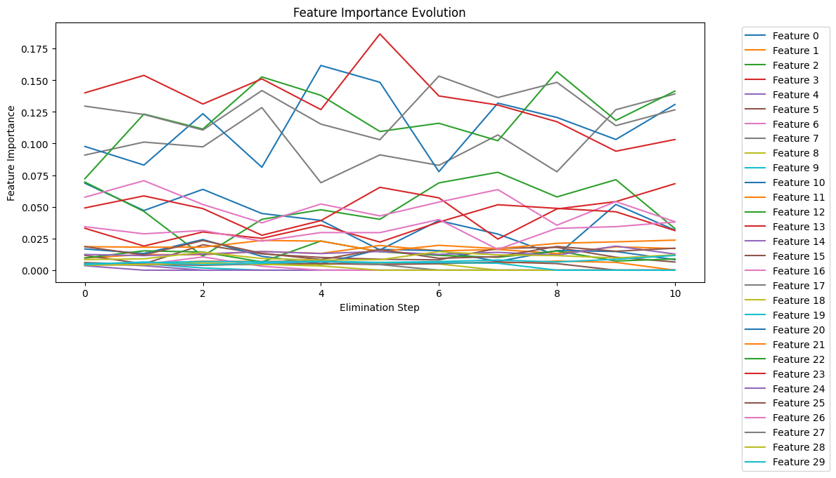
Fig 3: RFE Feature Importance Evolution
The plot above (refer to fig 3) shows how the importance of each feature changes as we eliminate features step by step. Let's break down what we're seeing:
The y-axis shows feature importance scores (0-0.175), while the x-axis shows elimination steps (0-10). Each colored line represents a different feature, and higher values indicate greater importance.
Several key patterns emerge from this visualization:
1. Dominant Features
- Several features (particularly Features 0-3) maintain consistently high importance (>0.125) throughout the process
- These features show resilience, suggesting they are crucial for the model
- The stability of their high importance scores validates their selection
2. Dynamic Changes
- Notice the spikes around steps 4-6, where some features suddenly gain importance
- This pattern often occurs when correlated features are removed, causing other related features to become more relevant
- Such shifts help us understand feature interactions
3. Feature Groups
- Top tier (>0.15): Features showing highest consistent importance
- Middle tier (0.05-0.15): Features with moderate importance
- Bottom tier (<0.05): Features that remain relatively unimportant throughout
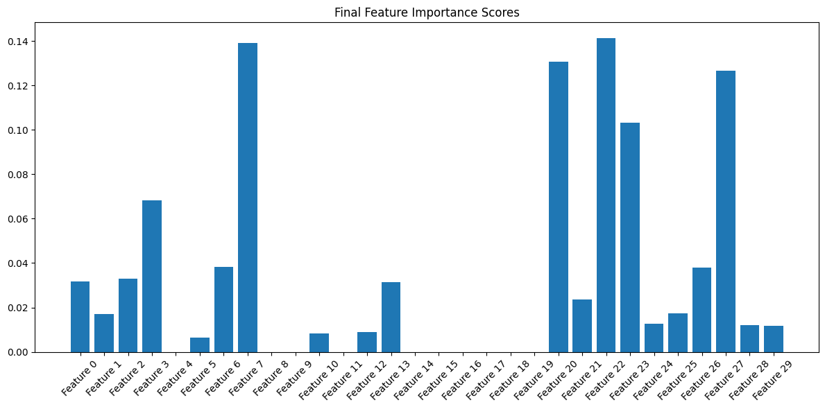
Building on our evolution analysis, the second visualization (Refer to Fig 4) provides a clear snapshot of our features' final importance scores. This bar plot helps us:
- Easily identify the strongest predictors
- See the relative differences between feature importance
- Confirm our evolutionary observations
- Verify that our selected features maintain significant importance
- Identify any potential outliers in our selection
How To Run the Code?
Step 1. Create a new Python file named rfe_implementation.py and copy all the code into it, including:
- All imports at the top
- All class and function definitions
- The main execution code under
if __name__ == "__main__":.
Step 2. Run the code:
python rfe_implementation.pyThis will automatically:
- Load the breast cancer dataset
- Run the feature selection process
- Print selected features
- Display stability scores
- Show visualizations of feature importance
Step 3. If you want to run the code on your dataset, you can do the following:
# Instead of using load_breast_cancer(), use:
X = pd.DataFrame(your_data)
y = your_target_variable
Optional parameters you can adjust:
- cv=5: Number of cross-validation folds
- n_iterations=10: Number of stability test iterations
- test_size=0.2: Train-test split ratio
- n_features_to_select: Number of features to keep
We’ve already seen the visualizations above. Now, let’s also have a look at the feature set after having applied RFE.
When applying RFE to the breast cancer dataset, we uncovered some fascinating patterns in how different measurements contribute to diagnosis. Let's break down what we found and what it means for practical applications.
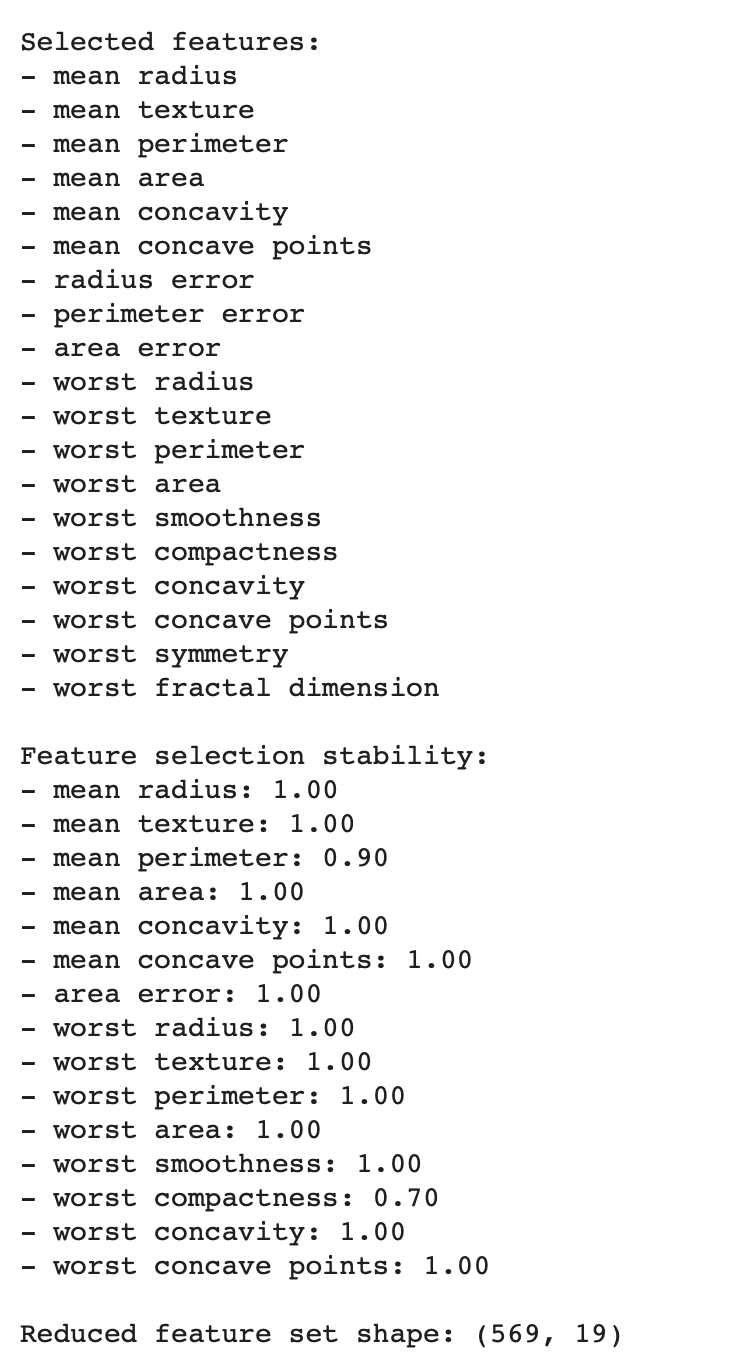
Our analysis started with a complex dataset of measurements from breast cancer samples. Through RFE, we managed to identify 19 key features that really matter for diagnosis (see fig 5).
- The majority of selected features show perfect stability (100% selection rate), which indicates high reliability in our feature selection process.
- Measurements related to radius, texture, and concavity were consistently selected across all iterations.
- The reduction from the original feature set to 19 features shows that we’ve successfully performed dimensionality reduction while maintaining key diagnostic indicators.
Conclusion
Throughout this guide, we've moved from theory to practice, using the breast cancer dataset to demonstrate how feature selection can make a real difference.
By reducing our feature set from 30 to 19 features, we maintained diagnostic accuracy while cutting computational overhead. We also discovered that measurements related to cell radius, texture, and concavity consistently emerged as reliable predictors across multiple test runs.
Here's what this means for your projects:
- Monitor your cross-validation scores closely as features are eliminated. This tells you exactly when to stop removing features.
- Always run at least 10 stability tests. One successful feature selection run could be luck; consistent results across multiple runs show you've found truly important features.
- Keep your visualizations handy. They show patterns and potential issues early.
The code we've worked through is ready for you to adapt. You can adjust the evaluation metrics to meet your specific needs or modify the stability thresholds to match your industry's standards.
Opinions expressed by DZone contributors are their own.
Comments