Visualizing Exposure Bias Using Simulation

Abstract

Randomization is a foundational assumption in A/B testing. In practice, however, randomized experiments can still produce biased estimates under realistic data collection conditions. We use simulation to demonstrate how bias can emerge despite correct random assignment. Visualization is shown to be an effective diagnostic tool for detecting these issues before causal interpretation.

Introduction

A/B testing is widely used to estimate the causal impact of product changes. Users are randomly assigned to control (C) or treatment (T), and differences in outcomes are attributed to the experiment. Randomization is intended to balance user characteristics across groups when assignment occurs at the user level. However, even with correct random assignment, the observed segment mix can differ because real experiments are often analyzed on a filtered or triggered subset of users. Eligibility rules, exposure conditions, logging behavior, and data availability can vary by variant due to trigger logic, instrumentation loss, device or browser differences, and latency. As a result, treatment and control may represent different effective populations.

This work examines how exposure bias can arise in such settings. The focus is not on flawed randomization but on how observation mechanisms distort the effective sample. We emphasize visualization as a first-line diagnostic.

Simulation Setup

For educational and diagnostic purposes, we construct a controlled simulation that mirrors a realistic website A/B testing environment. The objective is to understand how exposure bias can arise even when randomization is implemented correctly. From a causal inference perspective, this can be viewed as selection bias induced by conditioning on post-randomization exposure or triggering variables. In experimentation practice, this phenomenon is often referred to as exposure bias, because the imbalance arises from how users are observed rather than how they are assigned.

The core idea is to compare control (C) and treatment (T) behavior both before and after a trigger time for the same population of users. Under true randomization, there should be no systematic difference in click-through rate (CTR) between T and C prior to the trigger. Any pre-trigger difference indicates an imbalance that is unrelated to the treatment itself.

The simulation captures two features common in production experiments: heterogeneous user behavior and uneven exposure. Each run simulates 10,000 users observed over a one-week period. Impressions are simulated at the user level, and clicks are generated per impression. CTR is calculated as clicks/impressions. 

Users are assigned with equal probability to one of three behavioral segments defined by baseline click-through rate (CTR). One-third of users belong to a low-engagement segment with a mean CTR of 5%, one-third to a medium-engagement segment with a mean CTR of 10%, and one-third to a high-engagement segment with a mean CTR of 15%. Within each segment, individual CTRs vary around the segment mean with fixed variance. Segment assignment is independent of treatment assignment, so the underlying population is unbiased by construction.

In an ideal randomized experiment, roughly half of the users from each segment are assigned to treatment and half to control. Under this condition, aggregate CTR should be balanced between T and C before the trigger. In practice, however, the observed sample may deviate from this ideal. If a treatment contains substantially more or fewer users from a given segment, differences in CTR can appear even before the treatment is applied.

These pre-trigger differences are not caused by the treatment. They arise from differences in segment composition and will persist regardless of the intervention introduced in the treatment arm. If the analysis focuses only on post-trigger outcomes, such an imbalance can be incorrectly interpreted as treatment impact. Pre-trigger CTR comparisons are therefore informative only when exposure and metric definitions are consistent.

By varying the observed mix of low-, medium-, and high-CTR users between treatment and control, the simulation separates causal effects from composition effects. Aggregate CTR, therefore, depends on both the true treatment effect and the observed user mix.

A Jupyter Notebook is provided to support interactive exploration and visualization of these dynamics.

Simulation Scenarios and Visual Diagnostics

The table below pairs interpretation with visualization. The goal is not to estimate lift but to diagnose whether treatment and control still resemble samples drawn from the same population.

Visualization and Interpretation

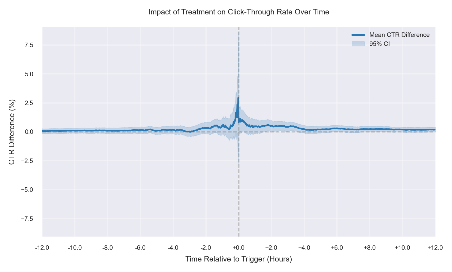
Case 1: Fully Randomized, No CTR Change Treatment and control are assigned uniformly across user segments, and no treatment effect is applied. The mean CTR difference (Treatment − Control) stays near zero both before and after the trigger, with the confidence interval consistently spanning zero. Any small fluctuations are consistent with sampling noise. This case is the ideal baseline for a healthy randomized experiment.
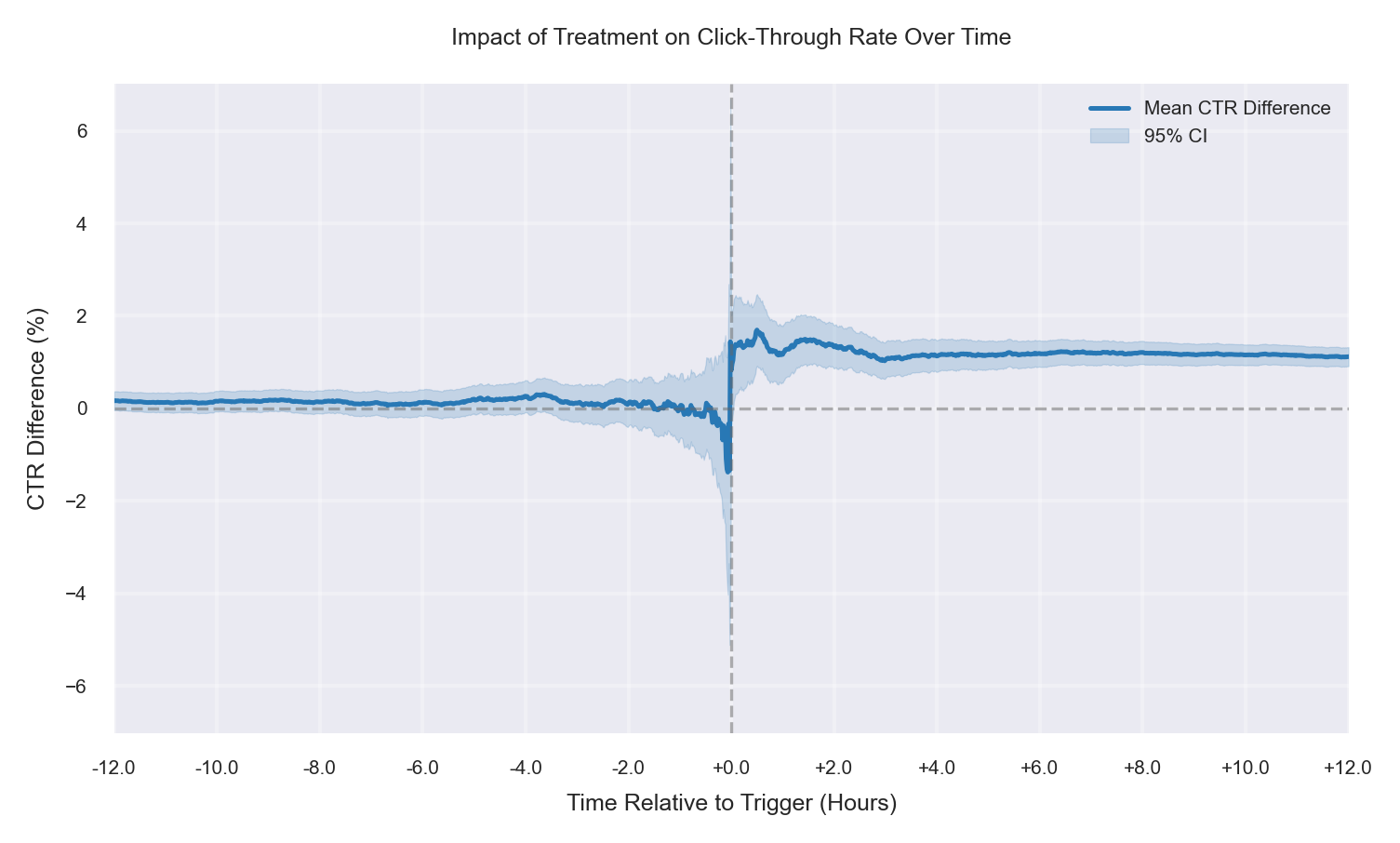
Case 2: Fully Randomized, +1% CTR Improvement Treatment and control remain balanced across segments, and a true positive treatment effect is applied. The mean CTR difference (Treatment − Control) is near zero before the trigger, then shifts upward after time 0 and stays positive, indicating a clean incremental lift. The pre-trigger alignment suggests no effective-sample mismatch, so the post-trigger change can be interpreted as a causal signal under correct randomization.
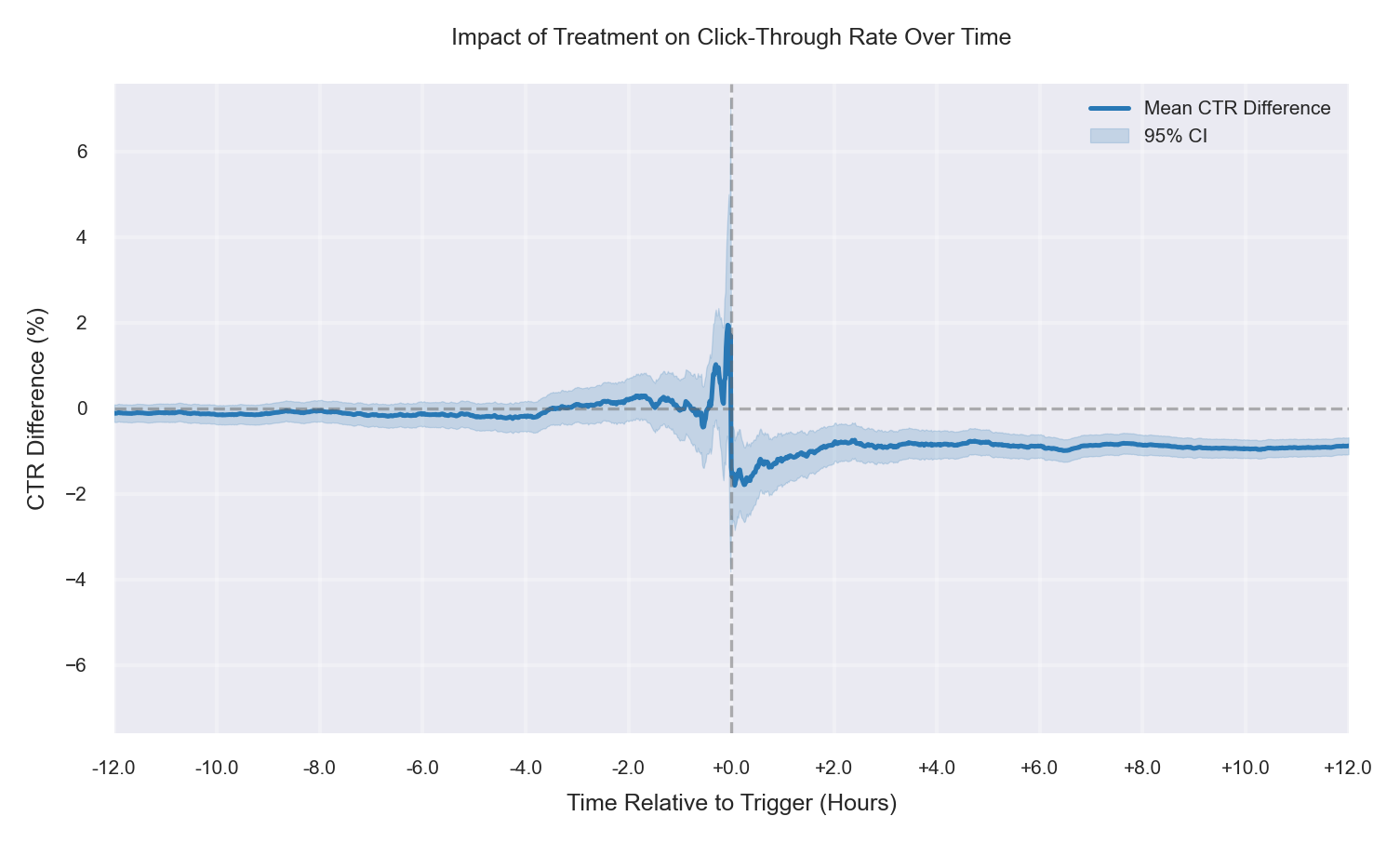
Case 3: Fully Randomized, −1% CTR Drop Treatment assignment is balanced across segments, but the intervention reduces CTR. The mean CTR difference (Treatment − Control) is near zero before the trigger, then shifts downward after time 0 and remains negative, indicating a clean post-trigger degradation. Because there is no meaningful pre-trigger offset, the observed drop can be attributed to the treatment under correct randomization.
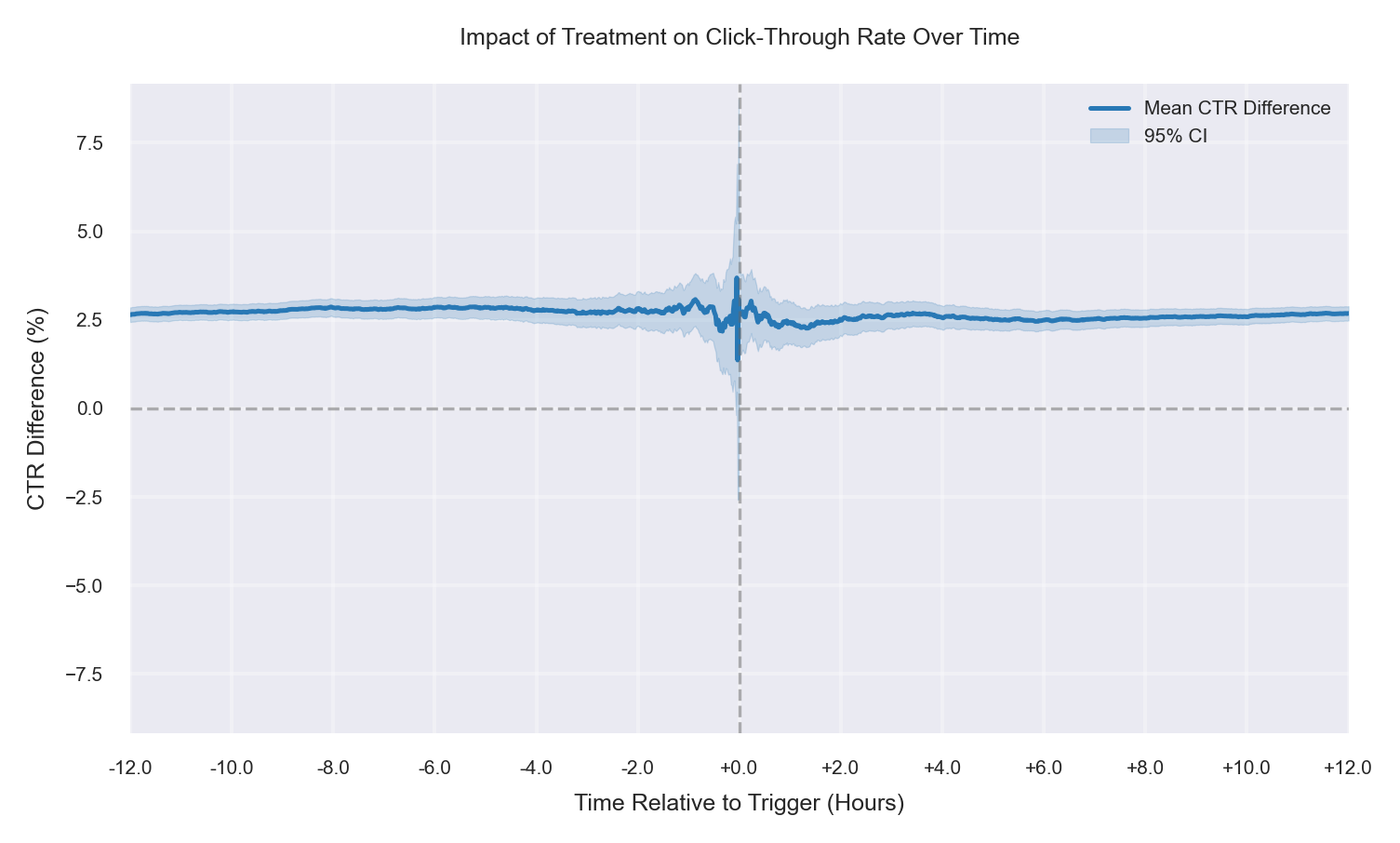
	Case 4: More High-CTR Users in T, No True Effect No treatment effect is applied, but the observed treatment sample contains a higher share of high-CTR users (segment mix imbalance). The mean CTR difference (Treatment − Control) is positive even before the trigger, and the post-trigger curve largely continues at the same offset with no additional shift. The apparent lift is therefore explained by segment composition (effective-sample mismatch), not a causal treatment effect.
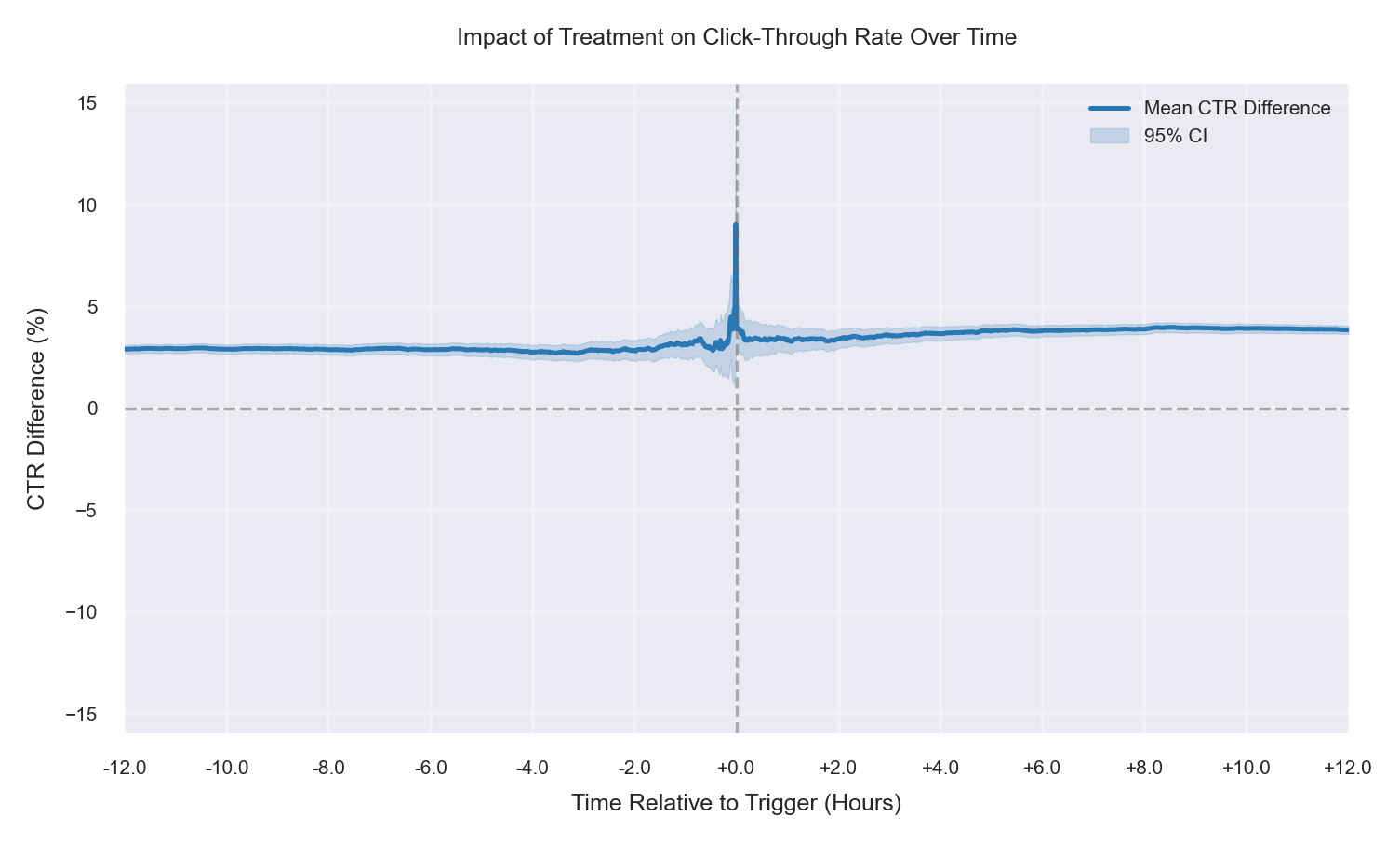
	Case 5: More High-CTR Users in T, +1% True Lift A true positive treatment effect exists, and the observed treatment sample also contains more high-CTR users (segment mix imbalance). The mean CTR difference (Treatment − Control) is already positive before the trigger (baseline offset), then increases further after time 0 (incremental treatment effect). As a result, the post-trigger lift overstates the true causal effect unless you account for the pre-trigger gap.
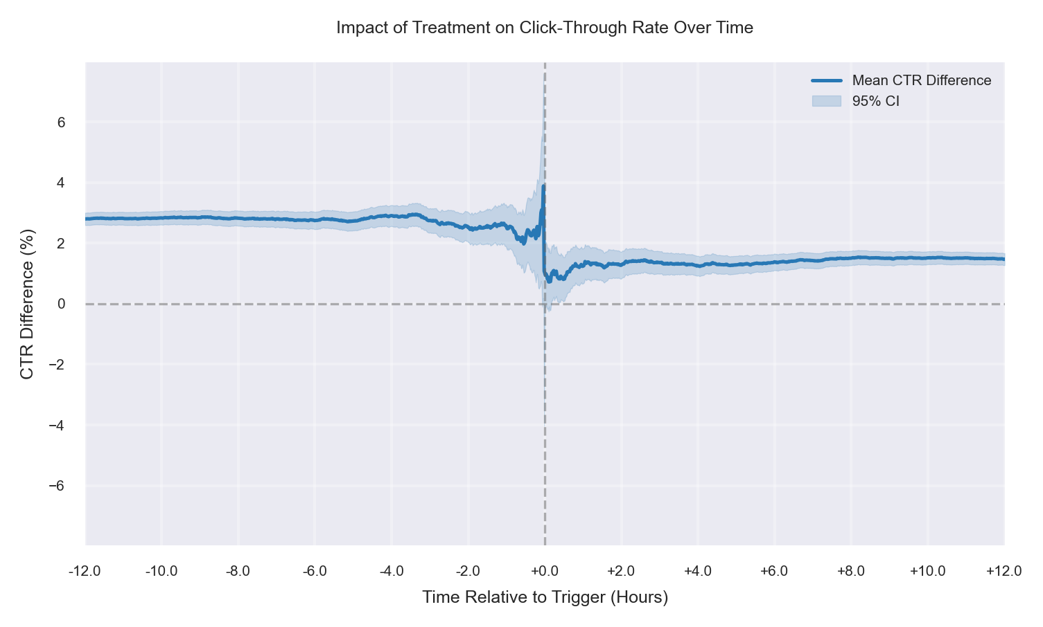
	Case 6: More High-CTR Users in T, −1% True Drop A true negative treatment effect exists, but the observed treatment sample contains a higher share of high-CTR users (segment mix imbalance). The mean CTR difference (Treatment − Control) is positive before the trigger, reflecting a baseline offset driven by composition. After time 0, the curve shifts downward due to the harmful treatment effect. Because the pre-trigger advantage partially (or even fully) cancels the post-trigger harm, the post-trigger result can look close to zero, only mildly negative, or even slightly positive—masking a real degradation behind composition bias.
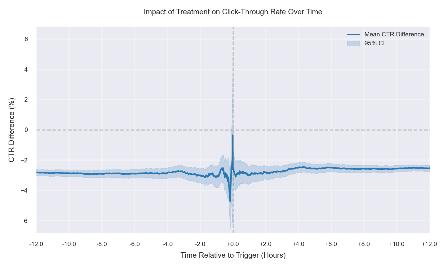
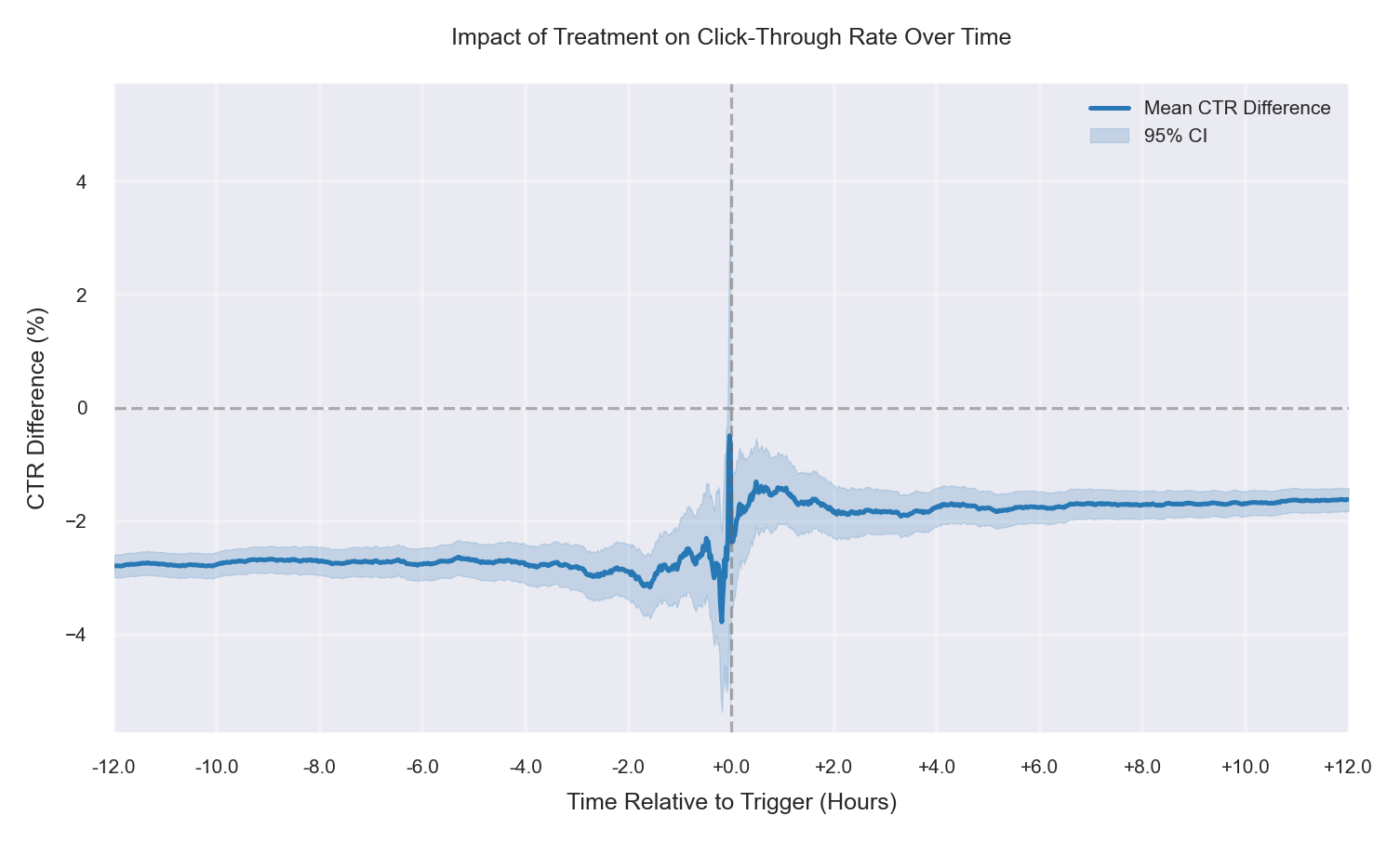
Case 7: More Low-CTR Users in T, No True Effect No treatment effect is applied, but the observed treatment sample contains more low-CTR users (segment mix imbalance). The mean CTR difference (Treatment − Control) is negative even before the trigger, indicating a baseline offset driven by composition. After time 0, the curve largely continues at the same level with no additional shift. The apparent degradation is therefore non-causal and explained by an effective-sample mismatch.
Case 8: More Low-CTR Users in T, +1% True Lift A real positive treatment effect exists, but the observed treatment sample is skewed toward low-CTR users (segment-mix imbalance). The mean CTR difference (Treatment − Control) is negative before the trigger (baseline offset), then shifts upward after time 0 due to the true lift. Because the post-trigger result combines both effects, the net lift can appear much smaller than the true causal improvement—or even look negligible—when interpreted without adjusting for the pre-trigger gap.
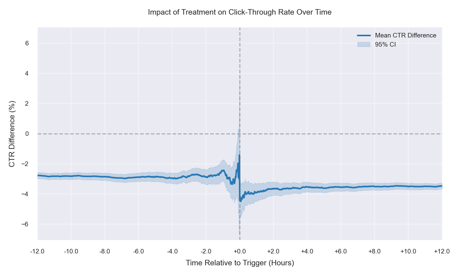
Case 9: More Low-CTR Users in T, −1% True Drop The treatment is genuinely harmful, and the observed treatment sample is also skewed toward low-CTR users (segment mix imbalance). The mean CTR difference (Treatment − Control) is already negative before the trigger (baseline offset), then shifts further downward after time 0 due to the true drop. Because composition bias and the causal effect move in the same direction, the post-trigger degradation is amplified—making treatment appear substantially worse than it truly is unless you adjust for the pre-trigger gap.

Conclusion

The simulations show that treatment and control can differ even before the trigger due to effective-sample composition (e.g., triggering/eligibility or logging differences). These baseline gaps can persist after the trigger and be mistaken for treatment effects. Visualization exposes this bias directly. Before interpreting CTR lift, verify that treatment and control still represent the same population.