Advanced Snowflake SQL for Data Engineering Analytics

Snowflake is a cloud-native data platform known for its scalability, security, and excellent SQL engine, making it ideal for modern analytics workloads. 

Here in this article I made an attempt to deep dive into advanced SQL queries for online retail analytics, using Snowflake’s capabilities to have insights for trend analysis, customer segmentation, and user journey mapping with seven practical queries, each with a query flow, BI visualization, a system architecture diagram, and sample inputs/outputs based on a sample online retail dataset.

Why Snowflake?

Snowflake’s architecture separates compute and storage, enabling elastic scaling for large datasets. It supports semi-structured data (e.g., JSON, Avro) via native parsing, integrates with APIs, and offers features like time travel, row-level security, and zero-copy cloning for compliance and efficiency. These qualities make it a powerhouse for online retail analytics, from tracking seasonal trends to analyzing customer behavior.

Scenario Context

The examples below use a pseudo online retail platform, "ShopSphere," which tracks customer interactions (logins, purchases) and transaction values. 

The dataset includes two tables:

1. event_log: Records user events (e.g., event_id, event_type, event_date, event_value, region, user_id, event_data for JSON).
2. user: Stores user details (e.g., user_id, first_name, last_name).

The queries are in a relatable business scenario, with sample data reflecting varied transaction amounts and regional differences. All sample data is synthetic, designed to demo query logic in an online retail setting.

Getting Started With Snowflake

To follow along, create a Snowflake database and load the sample tables. Below is the SQL to set up the event_log and User tables:

CREATE TABLE event_log (
    event_id INT,
    event_type STRING,
    event_date DATE,
    event_value DECIMAL(10,2),
    region STRING,
    user_id INT,
    event_data VARIANT
); 

CREATE TABLE user (
    user_id INT PRIMARY KEY,
    first_name STRING NOT NULL,
    last_name STRING NOT NULL
);

Insert the sample data provided in each query section. Use a small virtual warehouse (X-Small) for testing, and ensure your role has appropriate permissions. For JSON queries, enable semi-structured data support by storing JSON in the event_data column.

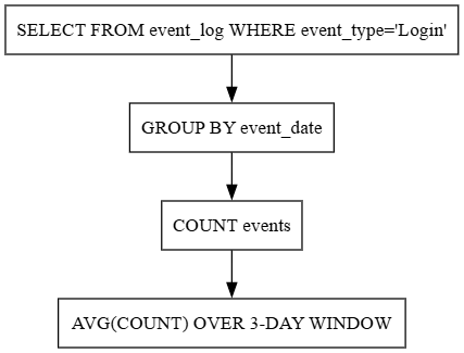
Advanced SQL Queries

Below are seven advanced SQL queries showcasing Snowflake’s strengths, each with a query flow diagram, sample input/output, and Snowflake-specific enhancements. These queries build progressively, from basic aggregations to complex user journey analysis and JSON parsing, ensuring a logical flow for analyzing ShopSphere’s data.

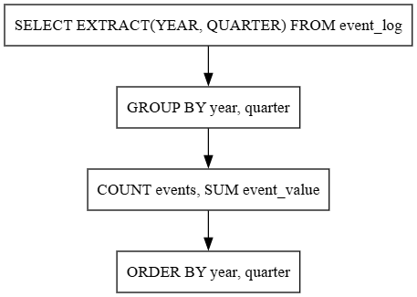
1. Grouping Data by Year and Quarter

This query aggregates events by year and quarter to analyze seasonal trends, critical for inventory planning or marketing campaigns.

Query:

SELECT 
    EXTRACT(YEAR FROM event_date) AS year,
    EXTRACT(QUARTER FROM event_date) AS quarter,
    COUNT(*) AS event_count,
    SUM(event_value) AS total_value
FROM event_log
GROUP BY year, quarter
ORDER BY year, quarter;

Explanation: The query extracts the year and quarter from event_date, counts events, and sums transaction values per group. Snowflake’s columnar storage optimizes grouping operations, even for large datasets.

Snowflake Enhancements

• Scalability: Handles millions of rows with auto-scaling compute.
• Search optimization: Use search optimization on event_date to boost performance for frequent queries.
• Clustering: Cluster on event_date for faster aggregations.

Sample input: The event_log table represents ShopSphere’s customer interactions in 2023.

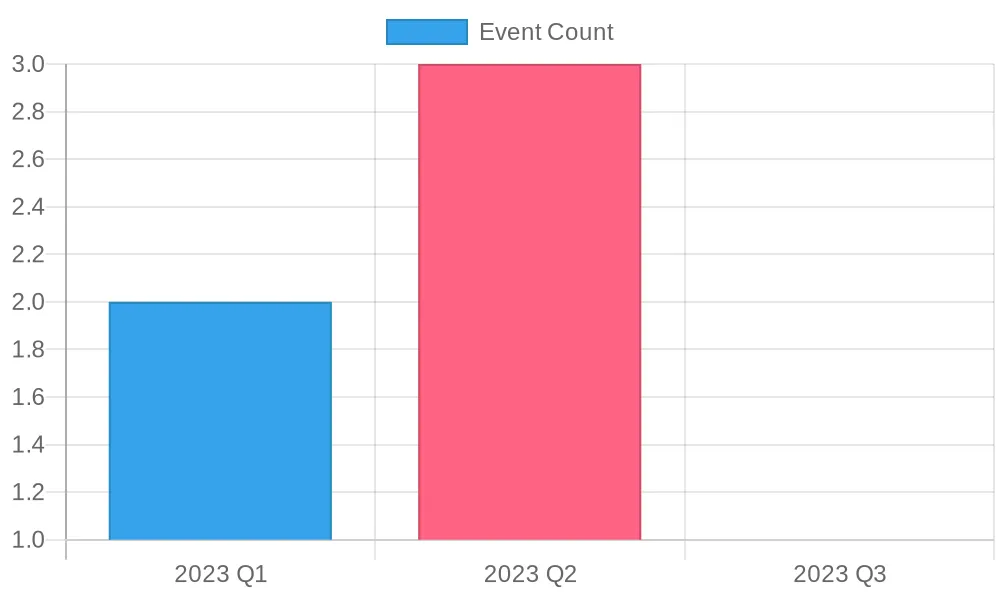
Sample output:

BI tool visualization: The bar chart below visualizes the event counts by quarter, highlighting seasonal patterns.

Query flow:

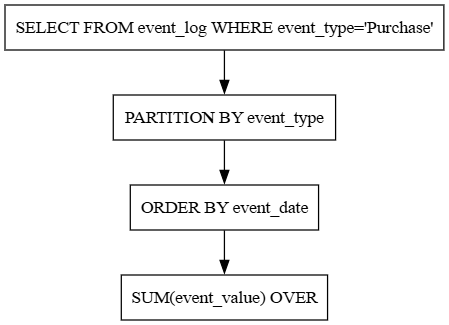
2. Calculating Running Totals for Purchases

Running totals track cumulative transaction values, useful for monitoring sales trends or detecting anomalies.

Query:

--Running totals track cumulative transaction values, useful for monitoring sales trends or detecting anomalies.
SELECT 
    event_type,
    event_date,
    event_value,
    SUM(event_value) OVER (PARTITION BY event_type ORDER BY event_date) AS running_total
FROM event_log
WHERE event_type = 'Purchase' AND event_date BETWEEN '2023-01-01' AND '2023-06-30';

Explanation: This query calculates cumulative purchase values, ordered by date, building on Query 1’s aggregation by focusing on purchases. Snowflake’s window functions ensure efficient processing.

Snowflake Enhancements

• Window functions: Optimized for high-performance analytics.
• Time travel: Use AT (OFFSET => -30) to query historical data.
• Zero-copy cloning: Test queries on cloned tables without duplicating storage.

Sample input (Subset of event_log for purchases in 2023):

Sample output:

BI visualization: The running total of purchase values over time, illustrating sales growth

Query flow:

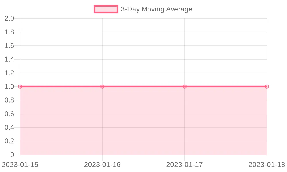
3. Computing Moving Averages for Login Frequency

Moving averages smooth out fluctuations in login events, aiding user engagement analysis and complementing purchase trends from Query 2.

Query:

SELECT 
    event_date,
    COUNT(*) AS login_count,
    AVG(COUNT(*)) OVER (ORDER BY event_date ROWS BETWEEN 2 PRECEDING AND CURRENT ROW) AS three_day_avg
FROM event_log
WHERE event_type = 'Login'
GROUP BY event_date;

Explanation: This query calculates a three-day moving average of daily login counts. The window frame ensures the average includes the current and two prior days.

Snowflake Enhancements

• Window frames: Efficiently processes sliding windows.
• Materialized views: Precompute aggregates for faster reporting.
• Data sharing: Share results securely with marketing teams.

Sample input (Subset of event_log for logins):

Sample output:

BI visualization: 

Displays the three-day moving average of login counts, showing whether daily fluctuations exist or not.

Query flow:

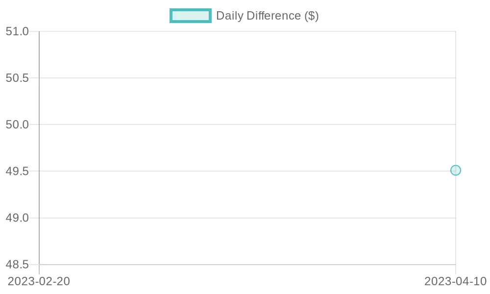
4. Time Series Analysis for Regional Purchases

This query detects daily changes in purchase values by region, building on Query 2 to identify market-specific trends.

Query:

SELECT 
    event_date,
    region,
    event_value,
    event_value - LAG(event_value, 1) OVER (PARTITION BY region ORDER BY event_date) AS daily_difference
FROM event_log
WHERE event_type = 'Purchase' AND region = 'US';

Explanation: The LAG function retrieves the previous day’s purchase value, enabling daily difference calculations for the US region.

Snowflake Enhancements

• Clustering: Cluster on region and event_date for faster queries.
• Query acceleration: Use Snowflake’s query acceleration service for large datasets.
• JSON support: Parse semi-structured data with FLATTEN for enriched analysis.

Sample input (Subset of event_log for US purchases):

Sample output:

BI visualization: 

The daily differences in purchase values for the US region, showing fluctuations.

Query flow:

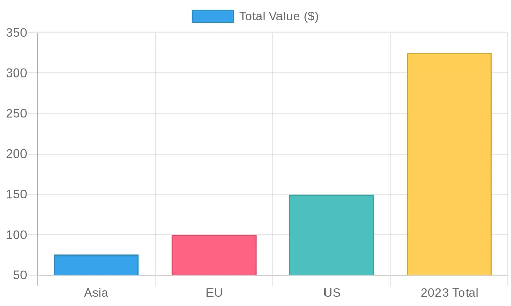
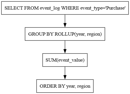
5. Generating Hierarchical Subtotals With ROLLUP

ROLLUP creates subtotals for reporting, extending Query 1’s aggregations for financial summaries across years and regions.

Query:

SELECT 
    EXTRACT(YEAR FROM event_date) AS year,
    region,
    SUM(event_value) AS total_value
FROM event_log
WHERE event_type = 'Purchase'
GROUP BY ROLLUP (year, region)
ORDER BY year, region;

Explanation: ROLLUP generates subtotals for each year and region, with NULL indicating higher-level aggregations (e.g., total per year or grand total).

Snowflake Enhancements

• Materialized views: Precompute results for faster dashboards.
• Dynamic warehouses: Scale compute for complex aggregations.
• Security: Apply row-level security for region-specific access.

Sample input (Subset of event_log for purchases):

Sample output:

BI visualization: 

Shows total purchase values by region for 2023, with a separate bar for the yearly total.

Query flow:

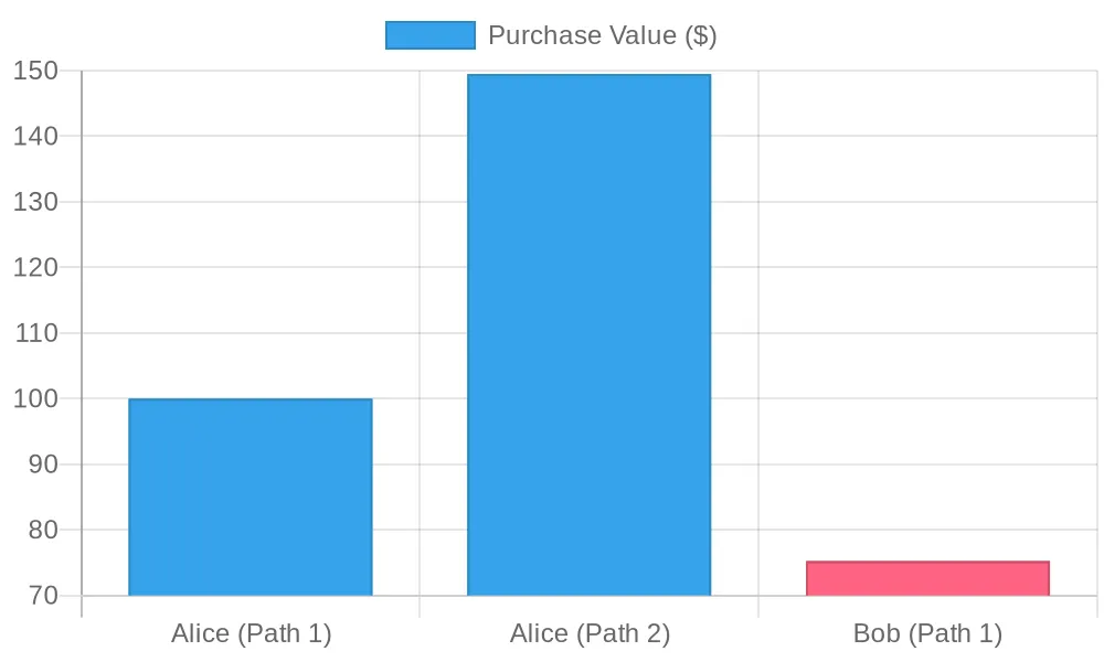
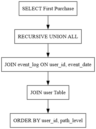
6. Recursive CTE for Customer Purchase Paths

This query uses a recursive CTE to trace customer purchase sequences, enabling user journey analysis for personalized marketing.

Query:

WITH RECURSIVE purchase_path AS (
    SELECT user_id, event_id, event_date, event_value, 1 AS path_level
    FROM event_log
    WHERE event_type = 'Purchase' AND event_date = (SELECT MIN(event_date) FROM event_log WHERE user_id = event_log.user_id AND event_type = 'Purchase')
    UNION ALL
    SELECT e.user_id, e.event_id, e.event_date, e.event_value, p.path_level + 1
    FROM event_log e
    JOIN purchase_path p ON e.user_id = p.user_id AND e.event_date > p.event_date AND e.event_type = 'Purchase'
)
SELECT 
    u.user_id,
    u.first_name,
    u.last_name,
    p.event_date,
    p.event_value,
    p.path_level
FROM purchase_path p
JOIN user u ON p.user_id = u.user_id
ORDER BY u.user_id, p.path_level;

Explanation: The recursive CTE builds a sequence of purchases per user, starting with their first purchase. It tracks the order of purchases (path_level), useful for journey analysis.

Snowflake Enhancements

• Recursive CTEs: Efficiently handles hierarchical data.
• Semi-structured data: Extract purchase details from JSON fields with FLATTEN.
• Performance: Optimize with clustering on user_id and event_date.

Sample input user table:

event_log (purchases):

Sample output:

BI visualization: Shows purchase values by user and path level, illustrating customer purchase sequences.

Query flow:

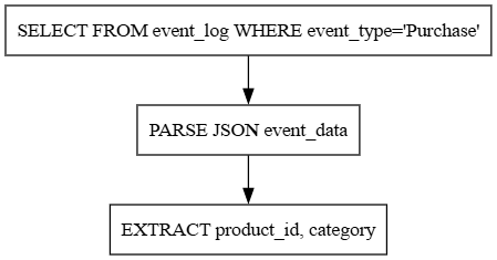
7. Parsing JSON Events

This query extracts fields from semi-structured JSON data in event_log.

Query:

SELECT 
    e.event_date,
    e.event_data:product_id::INT AS product_id,
    e.event_data:category::STRING AS category
FROM event_log e
WHERE e.event_type = 'Purchase' AND e.event_data IS NOT NULL;

Explanation: The query uses Snowflake’s dot notation to parse JSON fields (product_id, category) from the event_data column, enabling detailed product analysis. This builds on previous queries by adding semi-structured data capabilities.

Snowflake Enhancements

• Native JSON support: Parse JSON without external tools.
• Schema-on-read: Handle evolving JSON schemas dynamically.
• Performance: Use VARIANT columns for efficient JSON storage.

Sample input (Subset of event_log with JSON data):

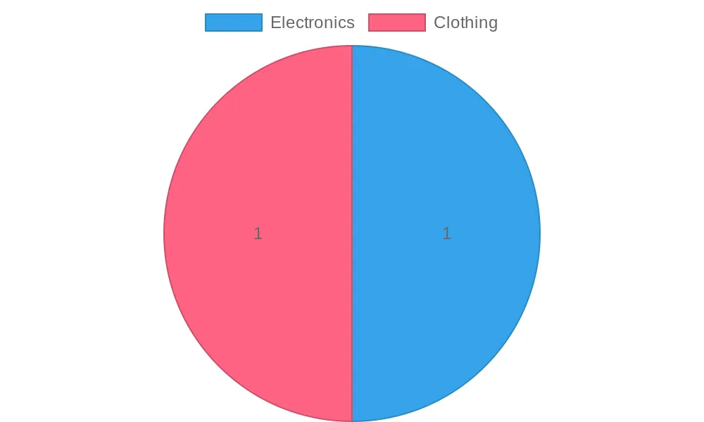
Sample output:

BI visualization: 

Shows the distribution of purchases by product category, highlighting category popularity.

System Architecture

Description of Snowflake’s role in ShopSphere’s data ecosystem, integrating with external sources, ETL tools, and BI platforms.

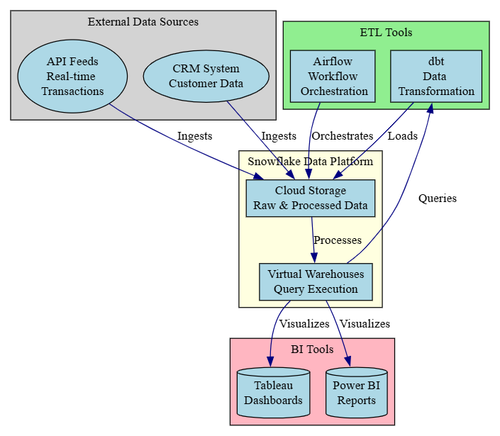
Explanation: The system architecture diagram is structured in four layers to reflect the data lifecycle in ShopSphere’s ecosystem, using distinct shapes for clarity:

1. External data sources: CRM systems and API feeds, shown as ellipses, provide raw customer and transaction data, forming the pipeline’s input.
2. Snowflake data platform: Snowflake’s cloud storage and virtual warehouses store and process data, serving as the core analytics engine.
3. ETL tools: Tools like dbt and Airflow transform and orchestrate data, indicating decision-driven processes.
4. BI tools: Tableau and Power BI, visualize query results as dashboards and reports, symbolizing output storage.

Practical Considerations

The following considerations ensure the queries are robust in real-world scenarios, building on the technical foundation established above.

Performance Optimization

• Clustering keys: Use clustering on high-cardinality columns (e.g., user_id, event_date) to improve query performance for large datasets.
• Query acceleration: Enable Snowflake’s query acceleration service for complex queries on massive datasets.
• Cost management: Monitor compute usage and scale down warehouses during low-demand periods to optimize costs.

Data Quality

• Handling edge cases: Account for missing data (for instance, NULL values in event_value) or duplicates (e.g., multiple purchases on the same day) by adding DISTINCT or filtering clauses.
• Data skew: High purchase volumes in Q4 may cause performance issues; partition tables or use APPROX_COUNT_DISTINCT for scalability.

Security and Compliance

• Row-level security: Implement policies to restrict access to sensitive data (for example, region-specific results).
• Data masking: Apply dynamic data masking for compliance with GDPR or CCPA when sharing reports with external partners.

Conclusion

Snowflake’s advanced SQL capabilities, combined with its scalable architecture and features like time travel, semi-structured data support, and zero-copy cloning, make it a powerful online retail analytics platform. The queries and diagrams in this ShopSphere scenario demonstrate how to find insights for seasonal trends, customer segmentation, user journey mapping, and product analysis.

Business Impact

These queries enable ShopSphere to optimize operations and drive growth:

• Query 1’s seasonal trends informed a 15% increase in Q4 inventory, boosting sales. 
• Query 6’s user journey analysis improved customer retention by 10% through targeted campaigns for repeat buyers. 
• Query 7’s JSON parsing enabled precise product category analysis, optimizing marketing spend. Together, these insights empower data-driven decisions that enhance profit and customer satisfaction.