ARIMA Forecasting With SAS

ARIMA stands for auto-regressive integrated moving average. It is also known as the Box-Jenkins model, as the ARIMA has been technique popularized by Box and Jenkins. For ARIMA forecasting, data needs to be stationary.

The ARIMA procedure analyzes and forecasts equally spaced univariate time series data, transfer function data, and intervention data by using auto-regressive integrated moving averages.

PROC ARIMA in SAS can be used to forecast.

Identification Stage

The Identification Stage computes auto-correlation, inverse autocorrelations, partial autocorrelations, and cross-correlations. Stationarity tests can be performed to identify whether differencing is necessary. It also provides descriptive statistics.

proc arima data=retail ;
   identify var=sales nlag=22;
run;

nlag controls the number of lags for which autocorrelation is shown. It should be always less than the number of observation in your dataset.

var is used to specify the name of the variable that needs to foreacst.

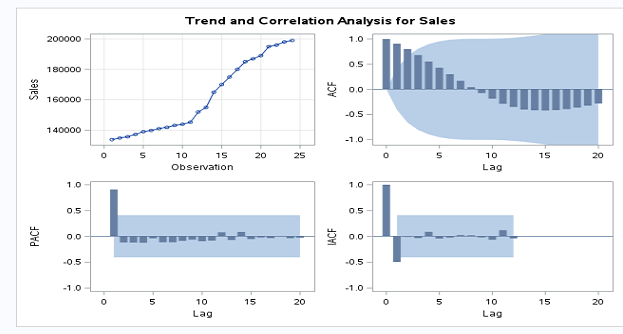
The identify statement produces panels of plots for auto-correlation and trend analysis.

• Time series plot of the series.

• Auto-correlation function plot (ACF).

• Inverse autocorrelation function plot (IACF).

• Partial autocorrelation function plot (PACF).

Differencing

If you plot sales, it seems that sales are changing from period to period. So data is non-stationary.

Now, we need to convert data into stationary data. It can be done as shown below.

proc arima data=LIBREF.FORECAST ;
   identify var=sales(1) nlag=22;
run;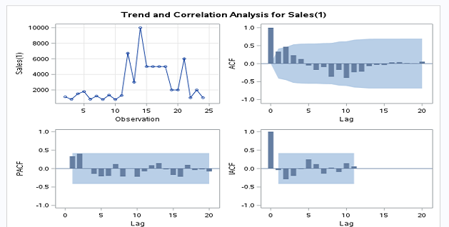

If we see the sales plot, it is non-stationary.

White Noise Test

In this case, white noise is rejected as a p-value for all lags less than or equal to 0.05. This is considered a good fit model.

Descriptive Statistics

The identify statement prints descriptive statistics for the sales series.

Estimation and Diagnostic Stage

The estimate statement is used to specify the ARIMA model to fit to the variable specified in the previous identify statement and to estimate the parameters of that model.

The estimate statement also produces diagnostic statistics to help you judge the adequacy of the model.

proc arima data = LIBREF.FORECAST;
identify var = Sales(1) nlag = 20 ;
estimate p = 1  q = 1;
run;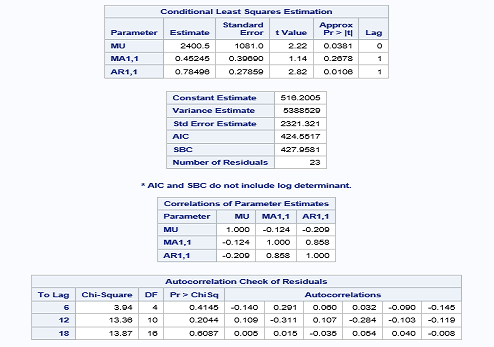

Forecasting Stage

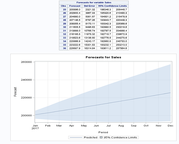
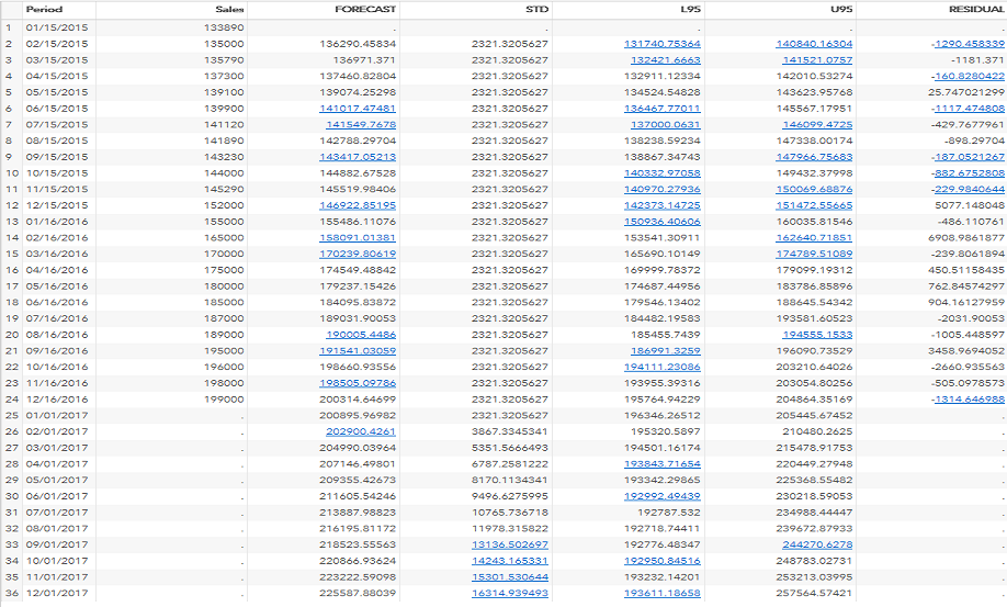
The FORECAST statement is used to forecast future values of the time series and to generate confidence intervals for these forecasts from the ARIMA model produced by the preceding ESTIMATE statement.

proc arima data = LIBREF.FORECAST;
identify var = Sales(1) nlag = 20 ;
estimate p = 1  q = 1;
run;
forecast lead=12 interval=month id=period out=results;
quit; 

• lead specifies how many period ahead to forecast. (12 months is our example).

• id specifies the ID variable (which is generally SAS date, time, and datetime).

• interval indicates the data are monthly.

• out allows us to write the forecast data to the datasets results.

Now, you know how to use the ARIMA model for forecasting.