How to Build ML Experimentation Platforms You Can Trust?

Machine learning models don’t succeed in isolation — they rely on robust systems to validate, monitor, and explain their behavior. Top tech companies such as Netflix, Meta, and Airbnb have invested heavily in building scalable experimentation and ML platforms that help them detect drift, uncover bias, and maintain high-quality user experiences.

But building trust in machine learning doesn’t come from a single dashboard. It comes from a layered, systematic approach to observability.

This article explores four core components of trustworthy ML experimentation:

1. Instrument everything you can
2. Real-time monitoring and anomaly detection
3. Shadow testing and replay pipelines
4. Statistical techniques to uncover hidden issues

1. Instrument Everything You Can

You can’t fix what you can’t see. And in production, that visibility starts with instrumentation. It helps teams understand how models, systems, and users behave by collecting key signals at every level: infrastructure-level metrics (CPU, memory, latency), application-level behavior (model predictions, user actions), and data statistics (feature distributions).

It’s a common practice in the industry today — most teams working on ML systems make sure to instrument every capability, from data pipelines to model predictions, so they can track issues end to end and understand what’s really happening in production.

Industry Systems in Action

• Netflix’s logging infrastructure: Captures billions of inference events asynchronously, ensuring low latency and broad visibility to monitor model behavior at scale without affecting user experience (Netflix Tech Blog).
• Meta’s ML observability platform: Logs every prediction, tracks feature distributions, monitors pipeline health, and uses feedback loops — enabling early issue detection and reliable performance at scale.

Best Practices

• Use versioned, strongly typed schemas (e.g., Protobuf, Avro)
• Include model version, timestamp, experiment ID, feature version, and request ID
• Store logs in immutable, queryable formats (e.g., Parquet in a lakehouse)

Extended Sample Log Format

A simplified model inference log might look like the following. This structure captures all the critical metadata needed for traceability, reproducibility, and future model improvement:

{
  "Version": "v01",
  "model_version": "linear_regression_v2",
  "request_id": "rId1",
  "features": {
    "device": "mobile",
    "age": "25",
    "similarity_score": "0.10",
    "feature_version": "f01"
  },
  "prediction_score": 0.78,
  "experiment_id": "exp42",
  "bucketId": "bucket101",
  "timestamp": 1721887245
}

Beyond detection, robust instrumentation supports:

• Root cause analysis of KPI drops
• Reproducibility across environments and model versions
• Improved retraining using logged inference inputs

2. Anomaly Detection and Real-Time Monitoring

After instrumentation is in place, the next step is to keep an eye on what’s happening as it happens. Real-time monitoring helps teams catch unexpected events, like a drop in conversion rates, an increase in model errors, or a slowdown in system performance. Anomaly detection adds another layer by flagging patterns that don’t match expected behavior. Together, they ensure issues are spotted early, so experiments can be paused or investigated before they cause bigger problems.

Industry Systems in Action

• Uber’s XP platform: Includes real-time metric tracking and automated anomaly detection.
• LinkedIn’s EKG and ThirdEye: Continuously scan experiment and infrastructure metrics. These tools compare treatment and control groups, flag anomalies, and generate alerts.
• Meta’s Hawkeye: Uses Jensen-Shannon divergence and SHAP analysis to detect drift in ranking models before silent failures impact users.

Best Practices

• Slice metrics by user segment (device, region, user tenure).
• Configure auto-alerts and automated rollback triggers.
• Track model performance drift using statistical divergence.

Here is a simple example of using Jensen-Shannon divergence to detect feature drift between training and live data distributions:

# Code Snippet 1

from scipy.spatial.distance import jensenshannon
import numpy as np

# Example feature histograms (e.g., device type counts)
# This could represent proportions of devices used during training vs. live usage
training_dist = [0.5, 0.3, 0.2]  # 50% mobile, 30% desktop, 20% tablet
live_dist = [0.3, 0.4, 0.3]      # 30% mobile, 40% desktop, 30% tablet

# Normalize distributions to sum to 1 (ensures valid probability distributions)
p = np.array(training_dist) / np.sum(training_dist)
q = np.array(live_dist) / np.sum(live_dist)

# Calculate the Jensen-Shannon divergence (a symmetric divergence metric)
js_div = jensenshannon(p, q) ** 2  # Square for interpretability on a 0-1 scale

# Trigger alert if drift exceeds threshold
if js_div > 0.01:
    print("Significant feature drift detected")

Jensen-Shannon divergence is symmetric, bounded between 0 and 1, and ideal for comparing categorical feature distributions like device types or regions.

You can also track SHAP drift to understand how a model’s reliance on features is changing over time:

The example below (code snippet 2) simulates a click prediction model for online ads, using features like ad position, type, and user device. By comparing SHAP summaries over time, you can detect if the model's reliance on certain ad formats or placements begins to drift, informing targeted investigation or retraining.

# Code Snippet 2 (note that this is a toy example using hardcoded data)
import shap
import pandas as pd
from sklearn.ensemble import RandomForestClassifier
from sklearn.model_selection import train_test_split

# Sample ad dataset: ad_position encoded as 1=top, 2=middle, 3=bottom
# user_device encoded as 0=mobile, 1=desktop
# clicked is the binary target variable

ad_data = pd.DataFrame({
    'ad_position': [1, 2, 3, 1, 2, 3],
    'user_device': [0, 1, 0, 1, 0, 1],
    'clicked': [1, 0, 1, 0, 1, 0]
})

# Define feature matrix and target vector
features = ad_data[['ad_position', 'user_device']]
target = ad_data['clicked']

# Split data into training set and live (test) set
features_train, features_live, target_train, target_live = train_test_split(
    features, target, test_size=0.5, random_state=42
)

# Train Random Forest classifier
rf_model = RandomForestClassifier(n_estimators=10, random_state=42)
rf_model.fit(features_train, target_train)

# Explain model predictions with SHAP
shap_explainer = shap.TreeExplainer(rf_model)
shap_values_live = shap_explainer.shap_values(features_live)[1]  # SHAP values for positive class (clicked)

# Calculate mean absolute SHAP values to assess feature importance
mean_abs_shap_values = abs(shap_values_live).mean(axis=0)
feature_names = features.columns

# Print summary of feature contributions
print("Average SHAP values for live data (clicked = 1):")
for feature_name, mean_shap_value in zip(feature_names, mean_abs_shap_values):
    print(f"{feature_name}: {mean_shap_value:.4f}")

3. Investigate With Shadow Testing and Replay Logs

Sometimes monitoring isn’t enough. You need tools to investigate issues more deeply and do it safely. That’s where shadow testing and replay logs come in.

What They Are

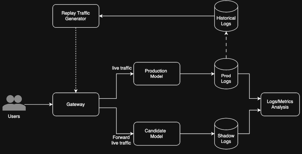
• Shadow testing: Runs real-time production traffic through both the current production model and a candidate model to compare predictions. This ensures the new model behaves as expected before rollout.
• Replay logs: Store historical inference data (inputs and outputs) so teams can re-run past traffic through updated models. This is crucial for debugging regressions and validating improvements.

Figure 1 below shows a realistic production setup where the live user traffic flows to both the Production Model and a Candidate Model via a Gateway. The Production outputs go to Prod Logs, while Candidate outputs go to Shadow Logs. Both are analyzed for differences in Logs/Metrics Analysis. Historical Logs power the Replay Traffic Generator to re-test models offline.

# Code Snippet 3

import pandas as pd
import matplotlib.pyplot as plt

# Create a DataFrame with ad performance by platform
data = pd.DataFrame({
    'Platform': ['iOS', 'iOS', 'iPad', 'iPad'],
    'Ad': ['Treatment', 'Control', 'Treatment', 'Control'],
    'Impressions': [1000, 100, 100, 1000],
    'Clicks': [50, 10, 20, 100]
})

# Calculate Click-Through Rate (CTR)
data['CTR (%)'] = data['Clicks'] / data['Impressions'] * 100

print("Platform-specific CTRs:")
print(data)

# Aggregate by Ad to simulate combined CTR across all platforms
aggregate = data.groupby('Ad')[['Impressions', 'Clicks']].sum().reset_index()
aggregate['CTR (%)'] = aggregate['Clicks'] / aggregate['Impressions'] * 100

print("\nOverall CTRs (aggregated):")
print(aggregate)

Platform-specific CTRs:
  Platform         Ad  Impressions  Clicks  CTR (%)
0      iOS  Treatment         1000      50      5.0
1      iOS    Control          100      10     10.0
2     iPad  Treatment          100      20     20.0
3     iPad    Control         1000     100     10.0

Overall CTRs (aggregated):
          Ad  Impressions  Clicks    CTR (%)
0    Control         1100     110  10.000000
1  Treatment         1100      70   6.363636

# Code Snippet 4
# SSRM: Sample Ratio Mismatch check
expected_ratio = 0.5       # Expected proportion of treated samples
threshold = 0.02          # Allowed deviation threshold (2%)
# Calculate actual ratio of treated samples
actual_ratio = treated / (treated + control)
# Check if deviation exceeds the threshold
if abs(actual_ratio - expected_ratio) > threshold:
    print("Sample ratio mismatch detected")

Conclusion: A Checklist for Trust

Trustworthy ML comes from a layered infrastructure, not just dashboards. Instrumentation, monitoring, shadow tests, and statistical analysis make experiments more reliable and actionable.

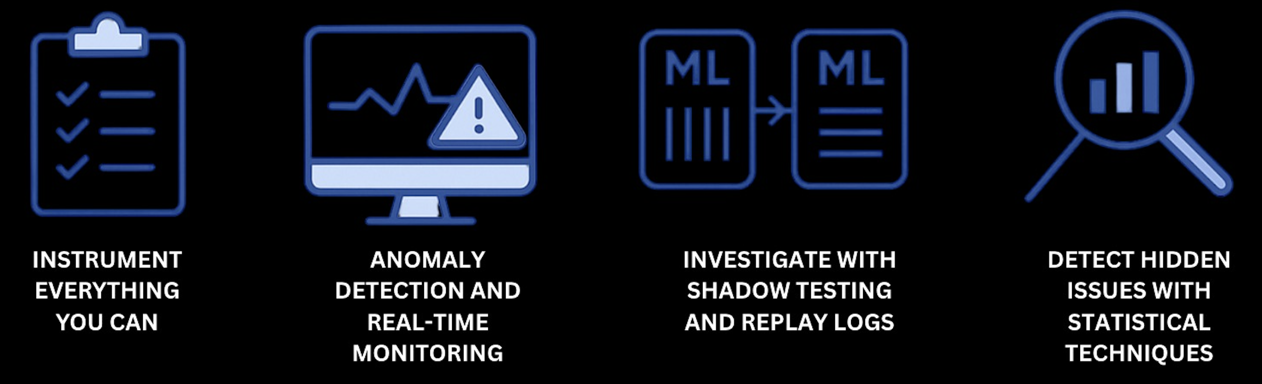
Before you go, use this quick checklist to put the core ideas into practice. Whether you’re starting from scratch or refining your stack, these steps help you build reliable ML experimentation across all four pillars.

1. Instrumentation

• Log inputs/outputs with model metadata.
• Use structured formats.
• Track feature and prediction distributions.

2. Monitoring

• Real-time dashboards with guardrails.
• Slice by key dimensions such as geography, device, and user type.
• Alert on drift (e.g., JSD, SHAP).

3. Shadow Testing and Replay

• Store historical logs for CI/CD replay.
• Set up shadow pipelines for candidate models.

4. Statistical Rigor

• Use CUPED, slice analysis, and SSRM.
• Visualize metrics by cohort.
• Build a culture of experimental validation.

Which of these layers would most strengthen your stack today?

Robust instrumentation, real-time monitoring, safe validation through shadow testing, and statistical rigor aren’t just best practices — they’re what separates trustworthy systems from fragile ones.