Designing Stop Loss in Modern AI-Driven Automated Trading Systems

From Rule-Based Algos to AI-Based Decision Systems

A decade ago, many electronic trading strategies were still mostly rule-based. You could often explain the logic in a few sentences. The systems were automated, but the decision rules were transparent and easy for humans to reason about.

Modern quantitative desks increasingly lean on machine learning and deep learning — and if we want to be a bit buzzwordy, we can call these AI-based trading systems. Models ingest high-dimensional order book data, news, and alternative data, and decisions are made by gradient-boosted trees, deep networks, or ensembles rather than hand-coded heuristics.

Two things change when you do that:

• The decision surface becomes harder to explain in plain English. Even the people who built the model may not be able to say exactly why it wants to buy or sell this instrument at this moment.
• The systems tend to operate in a much more fully automated fashion. Once you trust a model, you don’t want a human in the loop for every microsecond decision; you want it to stream orders all day, across hundreds of instruments and venues.

In that world, human judgment plays a less real-time role, but the cost of failure can be much higher. A mis-specified feature, a bug, or a regime change can push an AI-based strategy into regions of the state space it has never been designed for or seen before — and it will cheerfully keep trading unless something stops it.

That “something” is your risk-control architecture: the guardrails that sit around the model and define what’s allowed. Stop-loss rules are a frequent concept that traders employ, and almost any trading strategy design would mention stop-loss levels: If the performance of a trade or a strategy is -X%, exit that trade or even stop any further trading. Many treat such rules as inevitable components of any decent trading algorithm, especially in black-box AI-driven trading systems. This gives a feeling of safety, which sometimes can be false or even destructive, as engineering a stop loss can be prone to multiple design flaws, which we will show further in the article.

First, we will draw a line between two broad archetypes of trading firms and how they approach the problem of automated trading system design and stop-loss controls.

Trader-Centric vs. Quant-Centric System Designs

In modern quantitative trading, you can roughly split firms into two archetypes: trader-centric firms, where human traders are the primary decision-makers and “own” the PnL, and quant-centric firms, where quantitative researchers and their models are the primary decision-makers and the systems are expected to run with minimal human intervention.

In practice, most shops sit somewhere on a spectrum, but the distinction is useful because it drives how you design the trading system and its risk controls.

In trader-centric environments, the trading system is effectively a power tool for a human operator:

• Traders configure strategies, set risk limits, monitor order flow, market data, connectivity, positions, and trades throughout the day.
• They actively watch PnL and they’re expected to intervene: turn strategies off, hedge manually, or override misbehaving logic.
• The system is built with the assumption that a human is always there, looking at screens.

Because of this assumption, the engineering culture often tolerates a certain amount of known quirks and low-severity bugs. Some edge-case issues are consciously left unfixed if they’re rare, low impact, or expensive to address. If something strange happens (e.g., an ordering engine puts suboptimal quotes on one symbol, or the accumulated position does not correspond to the sum of trades registered in the database), the trader is expected to notice and correct it.

Alerting and monitoring exist, but rarely trigger some automated action to fix it, rather a signal to a human to pay attention.

Although in the age of proliferation of more advanced AI-driven systems, such setups become rarer, they still exist. This can be perfectly rational if you trade fewer products, have dense coverage of market hours by humans, and your business model explicitly values human judgment as part of the edge.

In quant-centric firms, the system design problem looks very different. The core assumption is that the system must be able to trade safely when nobody is watching it in real time.

You still have humans supervising and on call (often the role is called live-trading analyst), but they do not manually micromanage individual trades during the session, and usually cannot tweak the parameters of the strategy intra-day. Their primary authority is to hit a big red button: stop trading, reduce risk, escalate to owners.

That assumption drives a different set of requirements, with a much higher bar on correctness and robustness. Bugs that are annoying but fixable by a trader can be catastrophic if no one is watching. Replay or simulation frameworks become crucial components to reproduce the behavior of the trading system for any given period in the past. Let alone streamlined and centralized risk controls, comprehensive monitoring with actionable alerts, fallbacks, and fault tolerance.

In modern AI-driven algorithmic trading firms, this level of automation, monitoring, and central risk infrastructure is standard. The edge comes not just from the model itself, but from the ability to deploy many models safely across hundreds or thousands of instruments without watching each one manually.

This difference in system design is exactly where stop-loss logic comes in: in a trader-centric world, a stop loss might be implemented as “the trader will hit Ctrl+K if PnL is ugly enough.” In a quant-centric world, you need to be very explicit about what the machine should do, under which conditions, and how that interacts with the rest of your risk stack.

What Problem Is Your Stop Loss Actually Solving — More EV or Less Variance?

In an automated system, before you decide how to implement a stop loss, you should be clear about what problem it’s meant to solve.

When your edge comes from a machine learning or deep learning model, it’s tempting to think of the model itself as the whole story. In reality, the risk system around the model often determines whether the strategy is deployable at scale. In an AI-based system, a stop loss rule needs to be designed with the same level of care as the model training pipeline.

A good use of stop losses is when they serve as protection against non-model risk:

• Software bugs – incorrect ordering logic, miscounted positions, incorrect handling of the matching engine responses, etc.
• Market regime shifts – some structural changes in the market behavior that cannot be normalized and require a complete retraining of your model and strategy on new data.
• Black swan events – low-probability events with a drastic impact that can cause market shocks and liquidation spirals.
• Operational quirks and mistakes – exchange outages, latency spikes, wrong config pushed, incorrect parameter scale, strategy enabled on the wrong market.

For these, the main goal is to prevent the system from blowing up the account before a human even has a chance to understand what’s going on.

In that context, a stop loss can be chosen as some PnL change limit given statistical properties of the trading system, such as the PnL variance.

These stops are not about improving the system’s long-term profit, but bounding worst-case damage from extraordinary situations.

A different stop-loss use case is when the debate of improving the underlying edge arises. Motivation that can be frequently heard from traders and quants is that they believe a strategy has a positive edge on average, but want to cut losses in bad trades and let profits run.

This is where many practitioners mix up two completely different situations:

• Positive-edge strategy with painful variance and tail events. Here, stop-loss-like mechanisms can be sensible as long as they improve risk-of-ruin without destroying too much EV. Example: you cap extreme outliers to avoid account-level risk when the world goes off the rails.
• Negative-edge strategy dressed up with stop losses. No matter how fancy your stop logic is, if the underlying signal is on average losing money, thinking that you just need that one stop-loss rule to turn it to profit could be a fallacy. In backtests, you can often tune stop levels to make the past look better - but that’s just overfitting.

In fully automated shops, the approach tends to treat stop-loss rules as hypotheses: They must be tested via simulation and out-of-sample evaluation, and it’s never assumed that having a stop loss is inherently good. It might be negative EV once you account for noise, spreads, and fees.

Diagnosing Edge vs. Noise Before You Tune Stop Losses

Before you apply any stop logic, you should think if the strategy is generating positive expected value.

Let's consider some practical steps used at serious AI-driven trading firms:

• Look at distributions, not just equity curves.
  • Examine the distribution of trade-level or bar-level returns: mean, variance, skew, kurtosis, and tail behavior.
  • Check whether the mean is robust: does it persist across instruments, time periods, regimes?
  • If your base distribution is centered at or to the left of 0 after transaction costs, a stop loss will not magically create edge, it will just reshape the distribution.
• Run “unconstrained” and “constrained” simulations.
  • Build a simulation that runs your strategy without stop losses but with basic sanity checks (no insane leverage, no obviously unrealistic positions), and with candidate stop-loss rules.
  • Compare: EV of PnL, volatility, drawdown distribution, risk-of-ruin under your capital model.
  • If the unconstrained version is already negative on average, and your stop logic is the only thing making backtests look decent, you’re likely overfitting.
• One powerful diagnostic is to look at what happens after a hypothetical stop is event-studied on stop-loss triggers.
  • For every time your stop rule would have triggered, compute forward PnL over the relevant horizon (seconds, minutes, hours).
  • Aggregate those forward returns. If they’re mostly negative, your stop might be catching genuine “bad regimes” or model breakdowns. If they’re positive on average, your stop is likely just cutting mean-reverting noise and destroying EV.

Do You Actually Need a Stop Loss?

Let’s now be a little hands-on and move from theory to practical examples.

Below, we will introduce a couple of Python examples that illustrate a strategy with positive drift where a naive stop loss hurts EV (non-predictive stop) vs a regime-switching strategy where a stop loss protects you from a negative-drift regime (predictive stop).

Non-Predictive Stop Loss on a Positive-Edge Strategy

We model daily returns as i.i.d. normal with positive mean:

• mu > 0 (positive edge)
• some sigma (volatility)
• and a simple drawdown-based stop: if you lose more than X% from the peak, you liquidate and stay flat

import seaborn as sns
sns.set()

import numpy as np
import matplotlib.pyplot as plt


def simulate_equity(
    n_steps=500,
    mu=0.002,          # average daily return
    sigma=0.02,         # daily volatility
    stop_loss=-0.1,    # -10% max drawdown threshold
    seed=None,
):
    """
    Simulate one equity curve for a simple strategy with and without
    a naive stop-loss based on max drawdown.
    """
    rng = np.random.default_rng(seed)
    # i.i.d. daily returns
    rets = rng.normal(mu, sigma, size=n_steps)

    # Baseline: always in the market
    equity = np.ones(n_steps + 1)
    for t, r in enumerate(rets, start=1):
        equity[t] = equity[t - 1] * (1.0 + r)

    # With naive stop loss: if drawdown from peak <= stop_loss, go to cash and stay there
    equity_sl = np.ones(n_steps + 1)
    peak = equity_sl[0]
    in_market = True

    for t, r in enumerate(rets, start=1):
        if in_market:
            equity_sl[t] = equity_sl[t - 1] * (1.0 + r)
            peak = max(peak, equity_sl[t])
            drawdown = equity_sl[t] / peak - 1.0

            if drawdown <= stop_loss:
                # stop out and remain in cash
                in_market = False
        else:
            # stay in cash
            equity_sl[t] = equity_sl[t - 1]

    return equity, equity_sl


def monte_carlo(
    n_paths=2000,
    **kwargs,
):
    """
    Monte Carlo over many paths to estimate average terminal equity
    with and without the stop-loss rule.
    """
    finals = []
    finals_sl = []
    for i in range(n_paths):
        eq, eq_sl = simulate_equity(seed=i, **kwargs)
        finals.append(eq[-1])
        finals_sl.append(eq_sl[-1])
    return np.mean(finals), np.mean(finals_sl)


if __name__ == "__main__":
    # 1) Print average terminal equity
    base_ev, stop_ev = monte_carlo()
    print(f"Average terminal equity without stop loss : {base_ev:.3f}")
    print(f"Average terminal equity with naive stop   : {stop_ev:.3f}")

    # 2) Visualize a few sample equity curves
    n_paths_plot = 20
    curves_no_sl = []
    curves_sl = []

    for i in range(n_paths_plot):
        eq, eq_sl = simulate_equity(seed=i)
        curves_no_sl.append(eq)
        curves_sl.append(eq_sl)

    time = np.arange(len(curves_no_sl[0]))

    # 3) Build terminal equity distributions for histogram
    n_paths_hist = 2000
    finals = []
    finals_sl = []
    for i in range(n_paths_hist):
        eq, eq_sl = simulate_equity(seed=10_000 + i)
        finals.append(eq[-1])
        finals_sl.append(eq_sl[-1])
    finals = np.array(finals)
    finals_sl = np.array(finals_sl)
    mean_no_sl = finals.mean()
    mean_sl = finals_sl.mean()

    # 4) Plot: curves on the left, histogram on the right
    fig, (ax_curves, ax_hist) = plt.subplots(
        1,
        2,
        figsize=(12, 4),
        gridspec_kw={"width_ratios": [3, 1]},
    )

    # Left: sample equity curves
    for eq in curves_no_sl:
        ax_curves.plot(time, eq, color="g")  # solid: no stop-loss
    for eq_sl in curves_sl:
        ax_curves.plot(time, eq_sl, linestyle="--", alpha=0.4, color="k")  # dashed: with stop-loss

    ax_curves.set_xlabel("Time step")
    ax_curves.set_ylabel("Equity")
    ax_curves.set_title("Sample equity curves: no stop (solid) vs stop-loss (dashed)")

    # Right: terminal equity distributions + mean lines
    ax_hist.hist(
        finals,
        bins=30,
        alpha=0.6,
        label="No stop",
        density=True,
        color="g",
    )
    ax_hist.hist(
        finals_sl,
        bins=30,
        alpha=0.6,
        label="With stop",
        density=True,
        color="k",
    )

    ax_hist.axvline(
        mean_no_sl,
        linestyle="-",
        linewidth=2,
        color="g",
        label="Mean (no stop)",
    )
    ax_hist.axvline(
        mean_sl,
        linestyle="--",
        linewidth=2,
        color="k",
        label="Mean (with stop)",
    )

    ax_hist.set_xlabel("Terminal equity")
    ax_hist.set_ylabel("Density")
    ax_hist.set_title("Terminal equity distribution")
    ax_hist.legend()

    fig.tight_layout()
    plt.savefig(fname="naive_stoploss.png", dpi=300)
    plt.show()

Typical outcome when you run this:

Average terminal equity without stop loss : 2.749
Average terminal equity with naive stop   : 1.164

Without the stop, terminal equity has a healthy positive EV (because mu > 0). With the naive stop, EV drops significantly, because the stop is often triggered by normal volatility, and you never re-enter.

This is your non-predictive stop: it doesn’t know anything about future returns; it just cuts trades due to noise and pays spread/fees for the privilege.

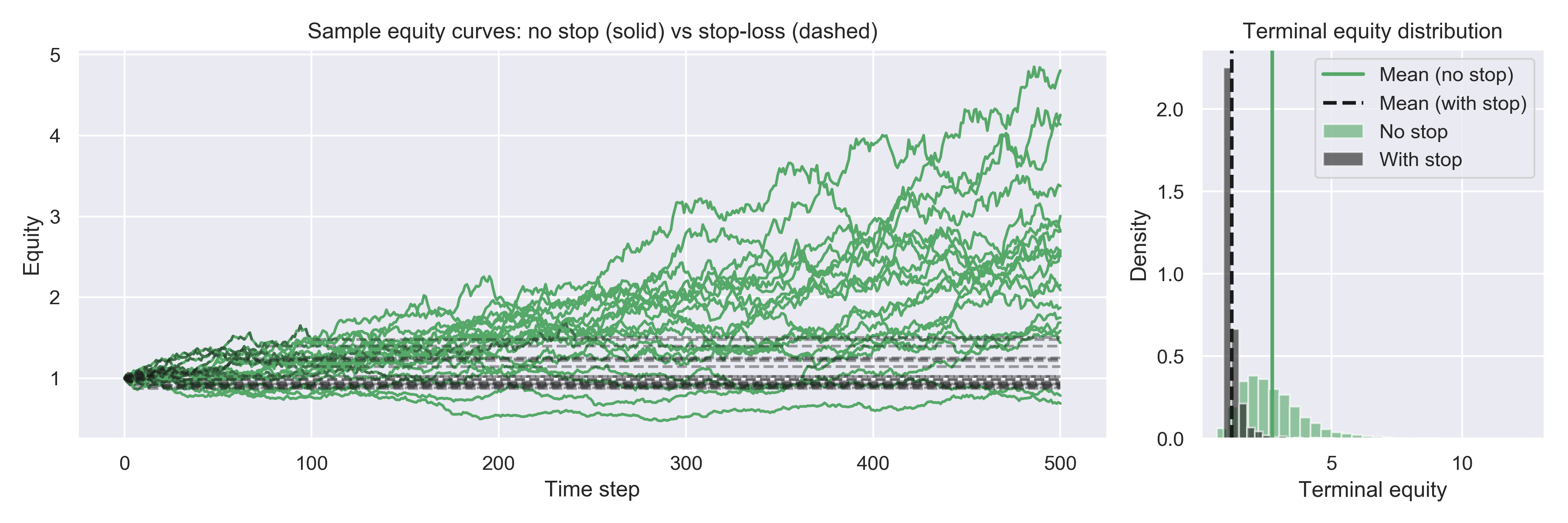
Figure 1: On the left: equity curves of several simulated strategies with a positive edge, in a scenario when no stop loss is used (green, solid) vs a naive non-predictive stop loss is used (black, dashed). On the right: distributions of the terminal equity (bars) with averages. We clearly see how a good trading strategy can be ruined: the stop systematically cuts off upside and lowers average terminal equity.

Predictive Stop Loss in a Regime-Switching World

Now we build a toy model where the process has:

• A good regime (positive drift mu_pos > 0),
• A bad regime (negative drift mu_neg < 0),
• A random switch between them somewhere in the middle of the trading period.

We simulate returns with a one-time switch from good to bad regime (suppose there is a fundamental change in the market microstructure that your model and strategy need to be retrained for). The stop loss doesn’t explicitly see the regime, but it reacts to drawdown; if the regime switch is severe enough, the stop will typically trigger early in the bad regime and keep us out of further losses.

import seaborn as sns
sns.set()

import numpy as np
import matplotlib.pyplot as plt


def simulate_equity_regime(
    n_steps=500,
    mu_pos=0.002,      # good regime drift
    mu_neg=-0.005,     # bad regime drift
    sigma=0.02,
    stop_loss=-0.1,    # -10% stop-loss
    seed=None,
):
    """
    Regime-switching example:
    - early period has positive drift (mu_pos),
    - later period has negative drift (mu_neg).
    We compare equity curves with and without a drawdown-based stop.
    """
    rng = np.random.default_rng(seed)

    # Choose a random switch time somewhere in the middle
    switch = rng.integers(low=int(0.3 * n_steps), high=int(0.7 * n_steps))

    rets_pos = rng.normal(mu_pos, sigma, size=switch)
    rets_neg = rng.normal(mu_neg, sigma, size=n_steps - switch)
    rets = np.concatenate([rets_pos, rets_neg])

    # Baseline: always in the market
    equity = np.ones(n_steps + 1)
    for t, r in enumerate(rets, start=1):
        equity[t] = equity[t - 1] * (1.0 + r)

    # With stop loss
    equity_sl = np.ones(n_steps + 1)
    peak = equity_sl[0]
    in_market = True

    for t, r in enumerate(rets, start=1):
        if in_market:
            equity_sl[t] = equity_sl[t - 1] * (1.0 + r)
            peak = max(peak, equity_sl[t])
            drawdown = equity_sl[t] / peak - 1.0

            if drawdown <= stop_loss:
                in_market = False
        else:
            equity_sl[t] = equity_sl[t - 1]

    return equity, equity_sl, switch


def monte_carlo_regime(n_paths=2000, **kwargs):
    finals = []
    finals_sl = []
    for i in range(n_paths):
        eq, eq_sl, _ = simulate_equity_regime(seed=i, **kwargs)
        finals.append(eq[-1])
        finals_sl.append(eq_sl[-1])
    return np.mean(finals), np.mean(finals_sl)


if __name__ == "__main__":
    # 1) Print average terminal equity in regime-switching world
    base_ev, stop_ev = monte_carlo_regime()
    print(f"Regime-switching – terminal equity without stop : {base_ev:.3f}")
    print(f"Regime-switching – terminal equity with stop    : {stop_ev:.3f}")

    # 2) Visualize a few sample equity curves
    n_paths_plot = 20
    curves_no_sl = []
    curves_sl = []
    switches = []

    for i in range(n_paths_plot):
        eq, eq_sl, switch = simulate_equity_regime(seed=i)
        curves_no_sl.append(eq)
        curves_sl.append(eq_sl)
        switches.append(switch)

    time = np.arange(len(curves_no_sl[0]))

    # 3) Build terminal equity distributions for histogram
    n_paths_hist = 2000
    finals = []
    finals_sl = []
    for i in range(n_paths_hist):
        eq, eq_sl, _ = simulate_equity_regime(seed=10_000 + i)
        finals.append(eq[-1])
        finals_sl.append(eq_sl[-1])
    finals = np.array(finals)
    finals_sl = np.array(finals_sl)
    mean_no_sl = finals.mean()
    mean_sl = finals_sl.mean()

    # 4) Plot: curves on the left, histogram on the right
    fig, (ax_curves, ax_hist) = plt.subplots(
        1,
        2,
        figsize=(12, 4),
        gridspec_kw={"width_ratios": [3, 1]},
    )

    # Left: sample equity curves
    for eq in curves_no_sl:
        ax_curves.plot(time, eq, linestyle="--", alpha=0.4, color="k")  # no stop-loss
    for eq_sl in curves_sl:
        ax_curves.plot(time, eq_sl, color="g")  # with predictive stop-loss

    ax_curves.set_xlabel("Time step")
    ax_curves.set_ylabel("Equity")
    ax_curves.set_title("Regime-switching equity: predictive stop-loss (solid) vs no stop-loss (dashed)")

    # Right: terminal equity distributions + mean lines
    ax_hist.hist(
        finals,
        bins=30,
        alpha=0.6,
        label="No stop",
        density=True,
        color="k",
    )
    ax_hist.hist(
        finals_sl,
        bins=30,
        alpha=0.6,
        label="With stop",
        density=True,
        color="g",
    )

    ax_hist.axvline(
        mean_no_sl,
        linestyle="--",
        linewidth=2,
        color="k",
        label="Mean (no stop)",
    )
    ax_hist.axvline(
        mean_sl,
        linestyle="-",
        linewidth=2,
        color="g",
        label="Mean (with stop)",
    )

    ax_hist.set_xlabel("Terminal equity")
    ax_hist.set_ylabel("Density")
    ax_hist.set_title("Terminal equity distribution")
    ax_hist.legend()

    fig.tight_layout()
    plt.savefig(fname="advanced_stoploss.png", dpi=300)
    plt.show()

Typical outcome:

Regime-switching - terminal equity without stop : 0.520
Regime-switching - terminal equity with stop	: 1.152

Without the stop, once you enter the negative-drift regime, you keep bleeding, so EV could go significantly below your starting capital. With the stop, you often cut the equity curve early in that regime, so EV is higher.

This is your predictive stop in the sense that “large drawdown” is correlated with “we’re likely in a bad regime”; the stop helps by preventing further negative EV.

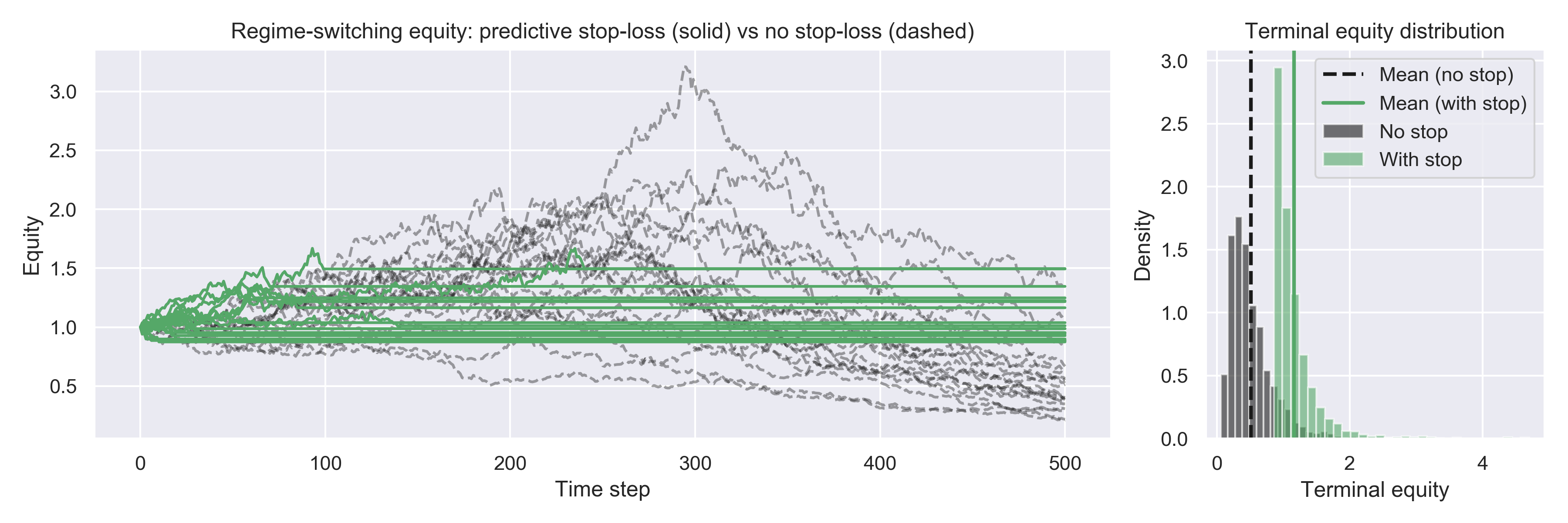
Figure 2: Regime-switching world – here the stop tends to trigger when we enter a bad regime, so the dashed curves and the histogram show higher terminal equity on average.

Closing Remarks

In modern trading systems, adding a stop loss is not a no-brainer, even when most of the trades are done by an AI-powered black box. Lots of practitioners are still prone to various fallacies while designing their trading pipelines.

A naive rule can silently destroy the edge of a good strategy by reacting to normal volatility, while a well-designed rule can materially reduce the risk of ruin in the presence of bugs, regime switches, and genuine model failures.

The key is to treat stop-loss logic as a design artifact you can test, not just a checkbox for (often false) safety and risk management.

First, convince yourself that your strategy has a positive edge before any stop logic, using distributional analysis and robust backtests. Then, evaluate any candidate stop rule empirically: How does it change EV, variance, drawdowns, and forward PnL after stop events? Finally, embed the rule into a layered risk architecture with clear ownership, monitoring, and safe failover.

That mindset is what lets highly automated shops run large books with relatively small teams, without relying on a human sitting in front of a screen to be their real stop loss.

Disclaimer: This article uses only publicly available information and is for informational and educational purposes only; it does not constitute investment advice. The views expressed are solely my own and do not represent those of my current or former employers or any other organization.