Dynamic Partition Pruning in Spark 3.0

With the release of Spark 3.0, big improvements were implemented to enable Spark to execute faster and there came many new features along with it. Among them, dynamic partition pruning is one. Before diving into the features which are new in Dynamic Partition Pruning let us understand what is Partition Pruning.

Partition Pruning in Spark

In standard database pruning means that the optimizer will avoid reading files that cannot contain the data that you are looking for. For example,

Select * from Students where subject = ‘English’;

In this simple query, we are trying to match and identify records in the Students table that belong to subject English. This translates into a simple form that is a filter on top of a scan which means whole data gets scanned first and then filtered out according to the condition.

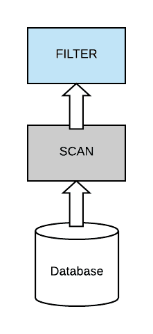
Now, most query optimizers try to push down the filter from the top of the scan down as close as possible to the data source, in order to be able to avoid scanning the full data set.

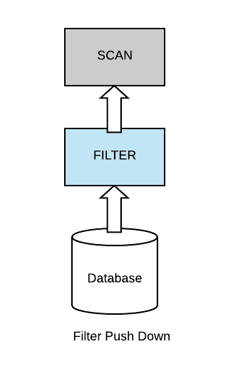
In the partition pruning technique, it follows the filter push down method and the data set is partitioned. Because in that case, if your query has a filter that’s on partition columns, you can actually be able to skip complete sets of partition files.

Partition pruning in Spark is a performance optimization that limits the number of files and partitions that Spark reads when querying. After partitioning the data, queries that match certain partition filter criteria improve performance by allowing Spark to only read a subset of the directories and files. When partition filters are present, the catalyst optimizer pushes down the partition filters. The scan reads only the directories that match the partition filters, thus reducing disk I/O.

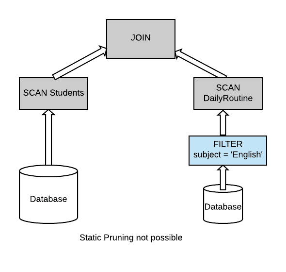
However, in reality data engineers don’t just execute a single query, or single filter in their queries, and the common case is that they actually have dimensional tables, small tables that they need to join with a larger fact table. So in this case, we can no longer apply static partition pruning because the filter is on one side of the join, and the table that is more appealing and more attractive to prune is on the other side of the join. So, we have a problem now.

xxxxxxxxxx

Select * from Students join DailyRoutine

where DailyRoutine.subject = ‘English’;

Some may suggest that we can join the dimension tables with the fact table beforehand. In this way, we can still trigger static pruning over a single table. And then, they can execute their filters in separate queries as shown below.

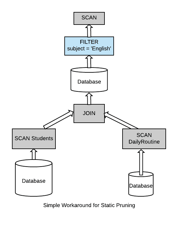
There are obvious downsides to this approach because first we have to execute this quite expensive join. We are duplicating the data, because we have to generate another intermediate table. This table can be quite wide because we take a bunch of smaller tables that we are joining together with a large table. And not only it’s wide but it’s actually extremely difficult to manage in the face of updating the dimensional tables. So whenever we are making a change we actually have to re trigger this whole pipeline over again.

In this blog we are going to learn a radically different approach in which we are going to do filtering using dynamic pruning. The basic goal of this optimization is to be able to take the filtering results from the dimension table. Then use them directly to limit the data that we will get from the fact table.

Dynamic Partitioning Pruning in Spark

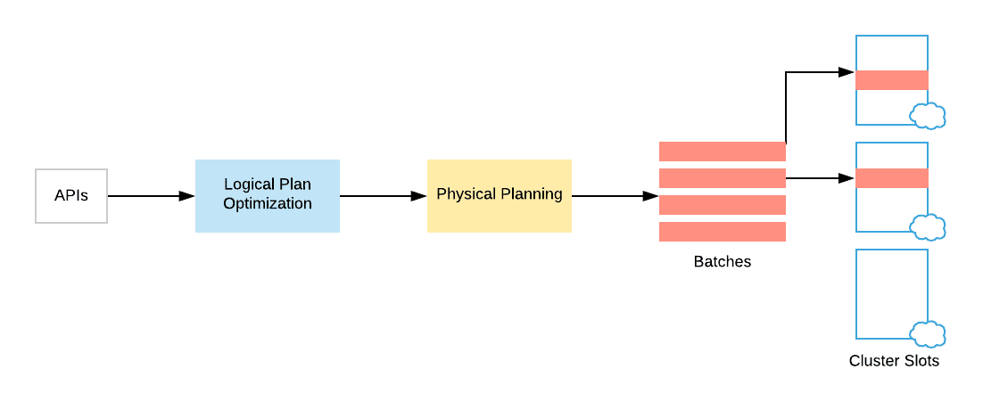
In Spark SQL, users typically submit their queries from their favorite API in their favorite programming language, so we have data frames and data sets. Spark takes this query and translates it into a digestible form, which we call the logical plan of the query. During this phase, Spark optimizes the logical plan by applying a set of transformations which are rule-based transformations such as column pruning, constant folding, filter push down. And only later on, it will get to the actual physical planning of the query.

During the physical planning phase spark generates an executable plan. This plan distributes the computation across clusters of many machines. Here I’m going to explain how dynamic partition pruning can be implemented at the level of logical planning. Then we will look into how we can further optimize it during physical planning.

Optimization at Logical Level

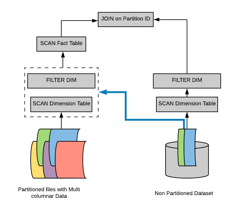
Let’s start with the optimization opportunities that we have at the level of logical planning. Let us consider a data set that is partitioned across multiple files. And each partition will be differ by a particular color. On the opposite side, we will have a smaller table, which is a dimension table that is not necessarily partitioned. And then we have the typical scan operators on top of these data sets. 

Whenever we are filtering the dimension table, consider an example in which only rows that correspond to two partitions on the opposite side of the join are actually relevant. So when we will complete the final join operation, only those two partitions will actually be retained by the join.

Therefore, we don’t need to actually scan the full fact table as we are only interested in two filtering partitions that result from the dimension table. To avoid this, a simple approach is to take the filter from the dimension table incorporated into a sub query. Then run that sub query below the scan on the fact table. 

And in this way we can figure out that when we are planning the fact side of the join. And we are able to figure out which data this join requires. This is a simple approach. 

But however it can actually be expensive. We need to get rid of this sub query duplication and figure out a way to do it more efficiently. In order to do that, we’re going to take a look at how spark executes a join during the physical planning and how Spark transforms the query during this physical planning stage.

Optimization at Physical Level

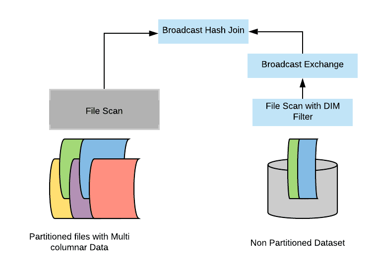
If the dimension table is small, then it’s likely that Spark will execute the join as a broadcast hash join. Whenever we have two tables that are hash joins, there are a number of things that are happening:

1. First, Spark builds a hash table out of the dimension table which we call the build relation.
2. After it executes this build relation, it will plug in the results of that side into a broadcast variable. Spark distributes that variable across all the workers that are involve in the computation. 
3. By doing so, we are able to execute the join without requiring a shuffle. 
4. Then spark will start probing that hash table with rows that come from the fact table on each worker node. 

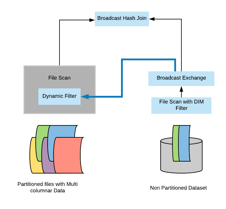
Now there is clearly a natural barrier between the two stages. So first, we are computing the broadcast side of the join. We are distributing it and only later on, do we start probing and executing the actual join. This is quite interesting, and we want to be able to leverage this into our optimization because this is quite exactly what we have mimicked with the level of logical planning with the sub query.

So here’s what we are actually going to do. We are intercepting the results of the build side – the broadcast results. And we are going to take them directly and plug them in as a dynamic filter inside the scanner on top of the fact table. So this is actually a very effective and optimized version of dynamic partition pruning.

Conclusion

To summarize, in Apache sparks 3.0, a new optimization called dynamic partition pruning is implemented that works both at:

1. Logical planning level to find the dimensional filter and propagated across the join to the other side of the scan.
2. Physical level to wire it together in a way that this filter executes only once on the dimension side.
3. Then the results of the filter gets into reusing directly in the scan of the table. And with this two fold approach we can achieve significant speed ups in many queries in Spark. 

I hope this blog was helpful.