From Dijkstra to A Star (A*), Part 2: The A Star (A*) Algorithm

Welcome back! If you missed Part 1 on the Dijkstra Algorithm, you can check it out here.

A* Algorithm

Could there be a way that, by using some clues, we could go straight to our destination and not visit other unnecessary nodes? Well, if we have some estimations, then yes, there is. If every node knows approximately how far down the shortest path the destination is, we can use this extra info, this estimation, to find our “road” faster. We call this a heuristic.

Using the heuristic we can build a function, f(n), that gives an estimation of the total path cost from the start node to the destination, if the current node, n, is on the path. We define it like this:

f(n) = g(n) + h(n)

Where:

• f(n) = total estimated path cost through node n
• g(n) = total path cost from start to n
• h(n) = estimated cost from n to the goal. The heuristic.

We can already calculate g(n), the total cost from start to n, using the Dijkstra algorithm, so, if we know h(n), we can get f(n), the estimated cost of the path through node n. In that case, we can change the Dijkstra algorithm to use this new function when getting the next node to visit from the frontier. This is A*.

A* is actually an informed variation of Dijkstra, where we use the estimation cost of the path through node n, the f(n) function, to choose the next node to visit. Having a good heuristic could help us to avoid visiting unnecessary nodes. It’s like having a hint where someone tells us, “use this way, is faster.” So, first we go that way, and if the hint is good, we will reach our goal faster.

Let’s change our previous implementation. We want to use the heuristic function when selecting the next node to visit from the frontier, thus transforming it in A*. The Edge object will be the same. It will have a target node and a cost associated it. Nothing changes here. In the Node class, we will add two new fields: h_cost and f_cost.

static class Node{

  public final String name;

  // cost so far to reach destination
  public double g_cost = Integer.MAX_VALUE;
  // total estimated cost of path through current node
  public double f_cost = Integer.MAX_VALUE;
  // estimated cost from this node to destination
  public final double h_cost;

  public List<Edge> adjacency = new ArrayList<>();
  public Node parent;

  public Node(String name, double h_cost){
    this.name = name;
    this.h_cost = h_cost;
  }

  public void addNeighbour(Node neighbour, int cost) {
    Edge edge = new Edge(neighbour, cost);
    adjacency.add(edge);
  }

  public String toString(){
    return name;
  }
}

The h_cost will be initialized by the constructor. It is the estimated cost to the goal node that we need to provide. The f_cost will be calculated by the A* algorithm based on g_cost and h_cost, and we will use it to select the next node to visit. Let’s see how:

public static void AStarSearch(Node source, Node destination) {
  source.g_cost = 0;
  // total estimated cost of path through current node will be in this case equal to h_cost
  source.f_cost = source.h_cost;

  PriorityQueue<Node> frontier = new PriorityQueue<>(new Comparator<Node>() {
    @Override
    public int compare(Node o1, Node o2) {
      return Double.compare(o1.f_cost, o2.f_cost);
    }
  });

  frontier.add(source);

  int numberOfSteps = 0;
  while (!frontier.isEmpty()) {
    numberOfSteps++;
    // get the node with minimum distance
    Node current = frontier.poll();

    System.out.println("Current node: " + current.name);

    // we have found the destination
    if (current.name.equals(destination.name)) {
      break;
    }

    // check all the neighbours
    for (Edge edge: current.adjacency) {

      Node neigh = edge.target;
      double cost = edge.cost;

      double new_g_cost = current.g_cost + cost;
      double new_f_cost = neigh.h_cost + new_g_cost;

      if (new_f_cost < neigh.f_cost) {
        neigh.parent = current;
        neigh.g_cost = new_g_cost;
        neigh.f_cost = new_f_cost;

        if (frontier.contains(neigh)) {
          frontier.remove(neigh);
        }

        frontier.add(neigh);
      }
    }
  }

  System.out.println("Number of steps: " + numberOfSteps);
}

So, if we look closely we see three differences from the previous algorithm:

• The PriorityQueue will compare the nodes based on the f_cost.
• We have to calculate a new f_cost based on the current estimated cost and the new g_cost.
• We update the best path so far, if the new f_cost is lower than the current f_cost.

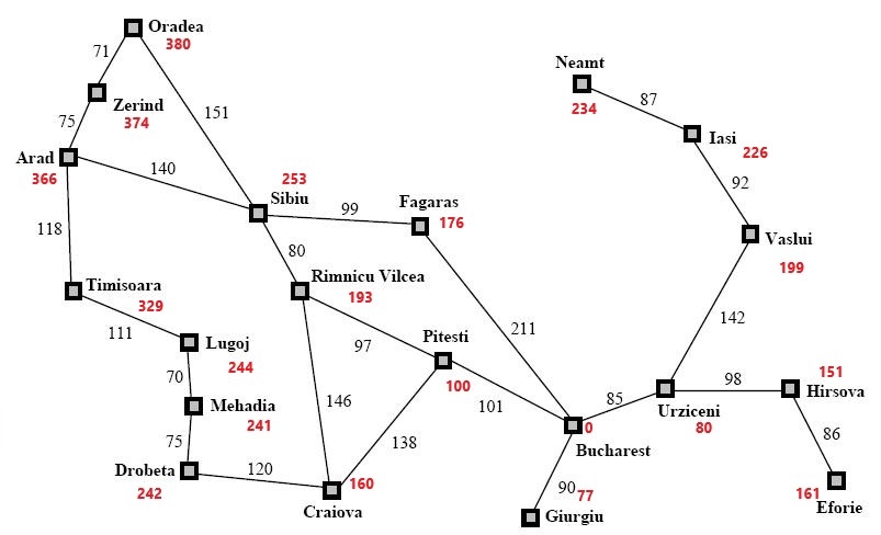
These are the only differences. All the other things remain the same. So, let’s see how it works. We are going back to our Romania map, but this time we add some heuristic info to each node in order to get an estimation on how long it would take to go from each city to Bucharest.

The estimation doesn’t need to be perfect, after all, is just an estimation. Of course, it is important to be as close to the real value as possible, but the important aspect here is to not overestimate and I will explain to you why a little later. For example, look at the Pitesti node. The real cost from Pitesti to Bucharest is 101, but the estimated value is 100. This will work. Let’s run our program on this map and let’s see what we get.

Current node: Arad
Current node: Sibiu
Current node: Rimnicu Vilcea
Current node: Fagaras
Current node: Pitesti
Current node: Bucharest
Number of steps: 6
Path: [Arad, Sibiu, Rimnicu Vilcea, Pitesti, Bucharest]

The efficiency is clear. We got the path just with 6 steps, instead of 13 steps that were necessary for the Dijkstra algorithm. Two times faster. It’s a huge improvement. (Actually, this doesn’t mean that A* is two times faster than Dijkstra. The optimization depends on the estimation accuracy).

So why is this working better? How did we go almost straight to Bucharest from Arad, with just one exception, Fagaras, and why didn’t we check the other nodes? Couldn’t we miss another and/or better path if we didn’t visit it? Well, this is because we select the next node to be visited based on the f_cost, that is:

f_cost = h_cost + g_cost

And, as I said before, the heuristic value should not be overestimated, that means that the heuristic function should be admissible. The h_cost should always be less than or equal to the real distance. Why? Well, our algorithm chooses the next node to visit based on the estimated value, and it will choose the node with the lowest f_cost.

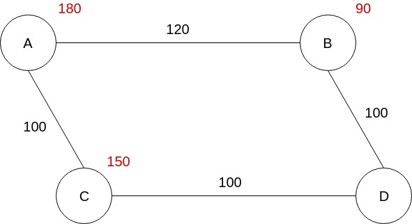
Let’s see a simple example where the h_cost is greater than the real cost and see what happens if the heuristic is not admissible.

In this graph, we see that the estimated cost from C to D is 150, and the real cost is 100. If we run our algorithm on this graph we will see that it calculates this shortest path, A -> B -> D, with a total cost of 220. But as you see, the path with the lowest cost is A -> C -> D, with a total cost of 200.

So why didn’t A* find the right path? Because it’s relying on the fact that the estimation is always less than or equal to the real value. So, if when picking a node to visit, the algorithm sees that the estimation is higher than the other node’s estimated value, why should it choose the first node? It will go with the second node, because, according to the admissibility condition, the real value can’t be lower than the estimated value, so it will not check that node. Thus, if the estimations don’t respect the admissibility condition, this algorithm will not function properly.

But, if the heuristics are admissible, the algorithm will work faster than the classic Dijkstra algorithm, because, it will check just the nodes that have the lowest f_cost, and given the fact that the f_cost  can’t be higher than the real path cost, we can be sure that we will not miss a better path. That’s why we see that, when traversing the Romanian map, it will go from Arad to Sibiu, Rm Valcea, without checking Oradea or Timisoara.

As you see, the algorithm will also check Fagaras, which is not on the shortest path, but the algorithm doesn’t know that yet. That’s because, after it visits the Rm Valcea node, the Fagaras node has an f_cost equal to 415 (g_cost = 239, h_cost = 176), and Pitesti has the f_cost equal to 417 (g_cost = 317 + h_cost = 100). So it will choose to visit Fagaras which has a lower estimated cost. After it visits it, it will see that the total cost from Arad to Bucharest through Fagaras is 450, while Pitesti has an f_cost equal to 415, so it will go to Pitesti, and it will continue to Bucharest, finding the shortest path.

Conclusion

So, in this article series, we saw how the Dijkstra algorithm works for helping us find the shortest path from one node to another. But, this algorithm left some room to improvement, so if we would have some estimated costs from each node to the destination, we can find the shortest path much faster. And this is how we transformed the Dijkstra algorithm into A star algorithm (A*).