A Guide to Developing Large Language Models Part 1: Pretraining

Recently, I came across a fascinating lecture by Yann Dubois in Stanford’s CS229: Machine learning course. The lecture offered an overview of how large language models (LLMs) like ChatGPT are built, covering both the fundamental principles and the practical considerations. I decided to write this article to share the key takeaways with a wider audience.

The five main components of LLM development are:

1. Architecture: The design of the network often based on transformers.
2. Training algorithms: How the model is trained to minimize loss.
3. Data: The quality, diversity, and relevance of training data.
4. Evaluation: Measuring progress and ensuring trained model meet goals.
5. Systems: Deploying large models on modern hardware to handle large computational demands.

LLMs such as ChatGPT, Claude, and Gemini have transformed AI, but their development goes far beyond the network architecture. While academia often focuses on architecture and training algorithms, this lecture emphasized the importance of data, evaluation methods, and systems optimization, areas that are crucial in practice but often overlooked in theory.

There are two main phases of developing an LLM:

• Pretraining: Or the language modeling phase, where a model is trained to understand and generate text based on web-scale datasets. An example of this is GPT-3.
• Post-training: This covers techniques like supervised fine-tuning (SFT) and reinforcement learning with human feedback (RLHF) to align models with user needs and make them effective AI assistants. Post-training is what allowed the development of ChatGPT from GPT-3.

This article is the first part of a two-part review and covers the first phase in LLM development, i.e., pretraining. It includes an overview of language modeling, evaluation, data, scaling laws, and practical considerations when building state-of-the-art (SOTA) models. Whether you’re a researcher, practitioner, or enthusiast, this overview will help you better understand what it takes to create these SOTA models.

Pretraining

1. Brief Overview of Language Modeling (LM)

Language modeling is at the core of pretraining LLMs. At a high level, a language model (LM) is a probability distribution over sequences of words or tokens. For example, given a sentence like "The mouse ate the cheese," the LM assigns a likelihood to the sentence based on its syntactic and semantic plausibility. It can recognize grammatical mistakes, like "The mouse ate cheese," or semantic inconsistencies, like "The cheese ate the mouse," and assign lower probabilities to such sentences.

Because an LM captures the probability distribution of text, it is a generative model, meaning it can generate new sentences by sampling from this distribution. This capability allows LMs to create coherent and contextually relevant text.

Currently, most LLMs, including those powering ChatGPT, are autoregressive language models. The key idea behind this approach is to break down the probability of a sentence,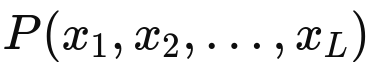using the chain rule of probability:

In simpler terms, the model predicts each word in the sequence based on the words that came before it, using the context to generate the next word.

• Pros: This method directly models the conditional probabilities of words, making it straightforward and effective for generating coherent text.
• Cons: When generating sentences, the model must loop through word-by-word predictions, conditioning on the words generated so far. For long sentences, this sequential process can slow down generation.

Despite these challenges, autoregressive models remain the standard for LLMs due to their ability to effectively model complex distributions of natural language. 

2. Autoregressive Language Models

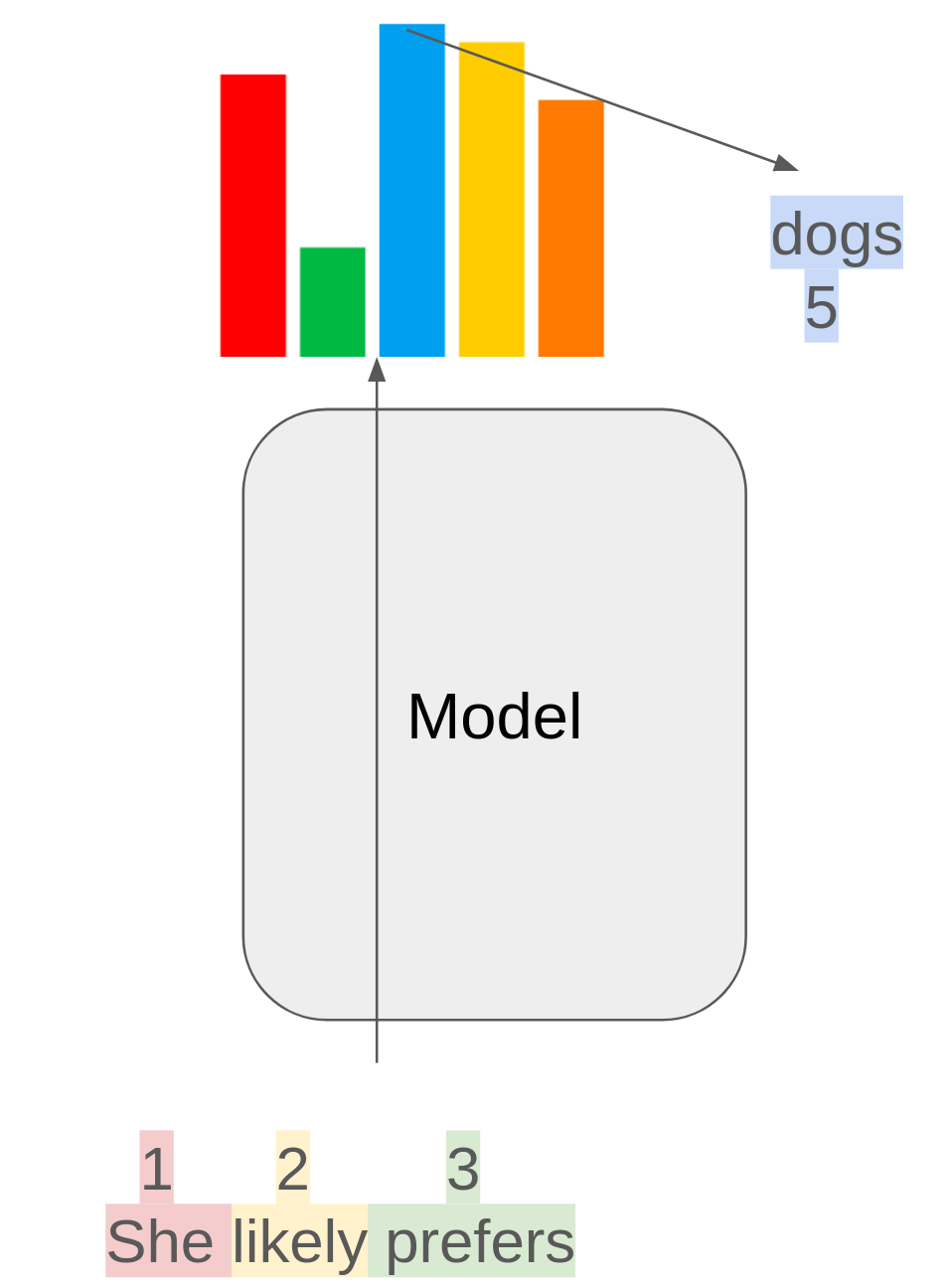
The primary task of these models is to predict the next word in a sequence based on the preceding context. For instance, given a partial sentence like "She likely prefers," the model might predict the next word as "dogs" with a certain probability.

Step-by-Step Working of an Autoregressive Language Model

1. Tokenization:
   • The input text is broken down into tokens (words or subwords), and each token is assigned a unique ID.
   • For example, the sentence "She likely prefers" might be tokenized as [1, 2, 3].
2. Embedding:
   • Each token ID is converted into a dense vector representation (embedding) that captures semantic and syntactic information.
3. Processing through the model:
   • The token embeddings are passed through a neural network (typically a transformer) to compute contextual representations for each token.
   • The model uses these representations to understand the relationship between tokens in the sequence.
4. Distribution over next token:
   • The model outputs a probability distribution over the entire vocabulary for the next token, conditioned on the given context.
   • This step involves a linear transformation of the contextual representation, followed by a softmax function.
5. Sampling (inference only):
   • A token is sampled from the probability distribution (usually the one with the highest probability).
   • The sampled token is detokenized back into a word or subword, forming the next part of the sequence.
6. Iterative generation (inference only):
   • The process repeats for subsequent tokens, with the context continually updated.

Training Autoregressive Models

During training, the model is tasked with classifying the next token based on the ground truth context. The main considerations here are:

• Loss function: The model uses cross-entropy (CE) loss, which compares the predicted probability distribution with the actual next token (represented as a one-hot encoded vector).
  • For example, if the actual next word is "cat," the one-hot vector would have a 1 at the index for "cat" and 0 elsewhere.
  • Cross-entropy loss minimizes the negative log likelihood of the correct token, which is equivalent to maximizing the text's overall log likelihood.

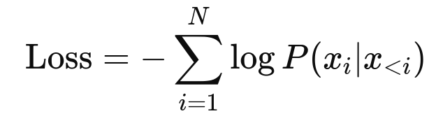Here, P(x_i | x_<i) is the model's predicted probability of token x_i, given all prior tokens in the sequence x_<i

• Output dimensionality: The final layer's output size equals the vocabulary size, ensuring a probability for each possible token.
• Role of tokenizers: While tokenizers are essential to autoregressive models, they are a vast field of study. We will briefly touch on this topic but skip many details for brevity.
  
  • The goal is to break text into tokens (manageable pieces) for model processing.
  • These are more general than words, allowing for variations like typos.

  • Approaches to tokenization:

    • Character-level tokenization: Fine granularity but results in very long sequences. Large computational overload because of O(N²) complexity
    • Subsequence tokenization: Groups text into frequently occurring subsequences (e.g., ~3 characters). Efficient balance between granularity and sequence length.

  • How subsequence tokenization works:

    1. Start with a character-level tokenizer.
    2. Iteratively merge common pairs of tokens in a large text corpus.
    3. Stop when the desired vocabulary size is reached or all tokens are merged.
    4. Apply the largest possible token at runtime for efficiency.

  • Challenges with tokenization:

    • Tokenizing specialized text (e.g., math, code) can be difficult. Models may not interpret numbers or syntax as humans do, requiring special tokenization strategies.

3. Evaluation

Perplexity

Perplexity measures the quality of a language model by assessing its ability to predict text. It is essentially the exponentiated average per-token loss, making it independent of the logarithmic base used. Perplexity can take values between 1 and L (length of vocabulary):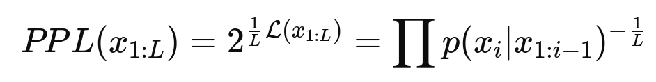

• Intuition: Represents the number of tokens the model "hesitates" between when predicting the next token. Lower perplexity indicates better performance. Historically, perplexity has improved significantly, from around 70 tokens in 2017 to fewer than 10 tokens today for SOTA models.
• Usage: Although perplexity is no longer a primary academic benchmark due to its dependence on tokenization and evaluation data, it remains an important metric for model evaluation.

Automatically Evaluatable Benchmarks

Using benchmarks consisting of tasks with clear, definitive answers (e.g., question-answering). E.g., HELM (Holistic Evaluation of Language Models), Huggingface Open LLM Leaderboard.

Academic Benchmarks

Focuses on academic rigor and tasks requiring diverse knowledge. E.g., MMLU (Massive Multitask Language Understanding) is widely used as a trusted pretraining benchmark.

Evaluation Challenges

• Sensitivity to prompting: Model performance can vary significantly based on the way prompts are structured.
• Inconsistencies: Outputs may lack consistency across similar tasks or inputs.
• Train-test contamination: In academia, ensuring no overlap between training and evaluation data is critical for fair assessment. In industry, this concern is less pronounced, as training data is typically well understood.

4. Data

Data is the most important part of training LLMs, yet it remains a highly challenging and evolving aspect. At a high level, it involves using the entirety of the internet or at least "clean" portions of it. However, this "clean internet" is poorly defined and far from representative of the desired outcomes for practical LLMs. 

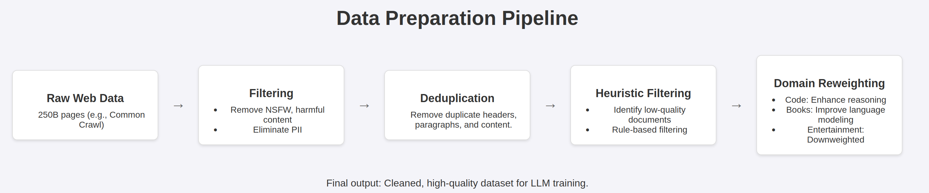
Key Steps in Data Collection and Preparation

1. Downloading the internet: Common Crawl is a widely used web crawler that captures approximately 250 billion webpages (~1PB of data). The main challenge here is extracting useful text from raw HTML, which often contains noisy elements like headers, footers, and incomplete sentences. Extracting math and technical content adds additional complexity.
2. Filtering undesirable content: Remove content that is NSFW, harmful, or contains personally identifiable information (PII). This is often done by blacklisting websites known for low-quality or harmful content. Or using models trained to classify and filter undesirable content.
3. Deduplication: To avoid repeated training on duplicate data.
4. Heuristic filtering: Rules based methods identify and remove low quality documents eg. those with outlier token distributions, abnormal text lengths (overly short or excessively long), suspicious content, such as gibberish or overly repetitive text.
5. Model-based filtering: We can use Wikipedia or other reputable sources and collect all links referenced by it. Then, train a classifier to predict whether a webpage could have been referenced by Wikipedia. This can be used to prioritize high-quality content similar to these references.
6. Domain classification and reweighting: Data is grouped into categories, such as code, books, and entertainment, and domain weights are adjusted based on their benefits. 
7. High-quality fine-tuning: Use learning rate annealing to "overfit" on this high-quality data, ensuring final refinements in the model.

Current Benchmarks and Datasets

• Open academic datasets:
  • C4: ~150B tokens (~800GB).
  • The Pile: ~280B tokens, containing diverse sources like ArXiv, PubMed Central, Stack Exchange, and GitHub.
  • Dolma: ~3T tokens.
  • FineWeb: ~15T tokens, the largest academic dataset.
• Closed models:
  • LLaMA 2: Trained on ~2T tokens.
  • LLaMA 3: ~15T tokens (aligned with the largest academic datasets).
  • GPT-4: Estimated at ~13T tokens.

Challenges and Open Questions

• Efficiency: How can we process massive datasets more efficiently? What new methods can reduce the computational overhead of filtering and deduplication?
• Balancing domains: How do we optimally balance data from various domains to achieve better downstream performance?
• Synthetic data: Can synthetic data generation complement or replace some training data, especially in underrepresented areas?
• Multimodal data: How can integrating text with other modalities (e.g., images, video) enhance performance, even on text-only tasks?
• Secrecy and legal issues: Companies frequently keep their data pipelines confidential to maintain a competitive edge. Additionally, publicly admitting to training on copyrighted materials, such as books, poses significant legal risks, making data collection strategies a sensitive and closely guarded aspect of LLM development.

5. Scaling Laws

Empirical studies have shown that increasing both the amount of data and model size leads to better performance. Scaling laws allow us to predict model performance based on the amount of data and the number of parameters.

Predicting Performance With Scaling Laws

A key insight from scaling laws is that when test loss is plotted as a function of compute, dataset size (in tokens), and parameters, the curve appears linear on a log-log scale. This means performance improvements can be estimated based on increased compute resources.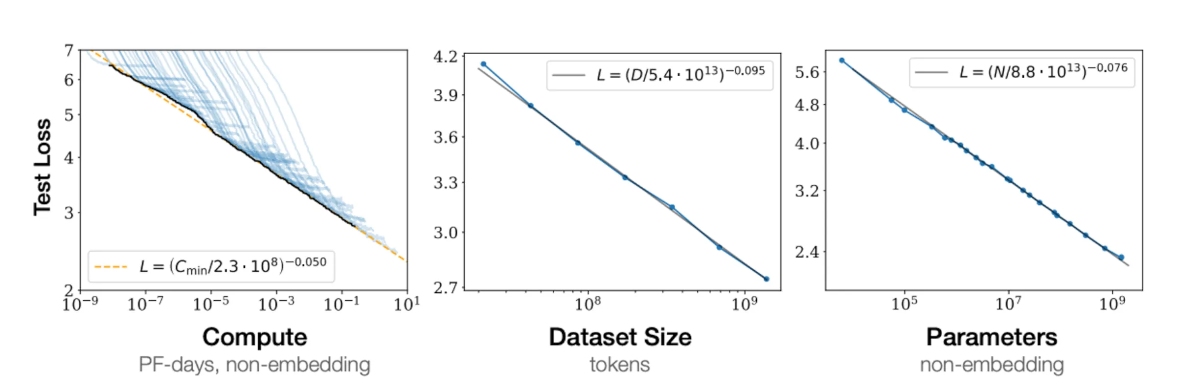

For example, we can ask, if we have access to 10,000 GPUs for one month, what is the best model to train given this constraint? Scaling laws provide a systematic way to answer this.
Old pipeline:

1. Tune hyperparameters on large models (~30 models)
2. Pick the best one
3. Train the final model for as long as the filtered-out ones (~1 day per model)

New pipeline:

1. Identify scaling recipes (e.g., learning rate adjustments as model size increases)
2. Tune hyperparameters on small models of varying sizes (~3 days)
3. Extrapolate performance using scaling laws
4. Train the final large model for the remaining time (~27 days)

Example use cases: 

• Model architecture selection: Suppose we need to choose between transformers and LSTMs. We train transformer models at various scales and plot their test loss. We do the same for LSTMs. By analyzing the scaling trends, we can determine which architecture will perform better at larger scales.
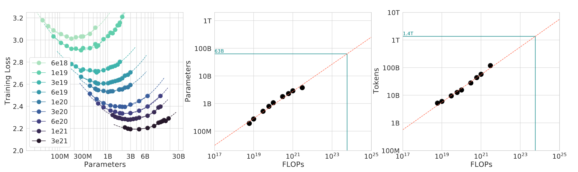
• Optimally allocating training resources: A critical question in large-scale training is balancing model size against the amount of training data. Chinchilla’s findings suggest an optimal token-to-parameter ratio of 20:1 for training. When accounting for inference, the ideal ratio increases to 150:1. To determine the best allocation of compute, we can plot isocurves, which show models trained with the same amount of compute while varying model size and dataset size. By analyzing these curves, we can identify the best model size for a given compute budget.

Scaling laws help answer several critical questions:

• Resource allocation: Should we train longer or use bigger models? Should we collect more data or invest in additional GPUs?
• Data considerations: Should we train with multiple epochs or focus on diverse data? How should we weigh different data sources?
• Algorithmic choices: Should we use transformers or LSTMs? Should we prioritize model width or depth?

The Bitter Lesson

Larger models trained with more data consistently outperform smaller, finely-tuned architectures. Avoid overcomplicating models. Focus on simple, scalable architectures and leverage computational growth effectively.

6. Training a SOTA Model

SOTA models require vast computational resources, and recent large-scale models like LLaMA 3 (405B parameters) provide a useful benchmark for estimating training costs. Below is a breakdown of key training metrics and resource consumption for such models.

Training Data and Compute Scaling

LLaMA 3 was trained on 15.6 trillion tokens, achieving an optimal tokens-to-parameters ratio of ~40, which is considered training compute optimal based on scaling laws. This balance is crucial for efficiency and performance.

The training FLOPs can be estimated using the approximation:

where N is the number of tokens and P is the number of parameters. For LLaMA 3, this is:

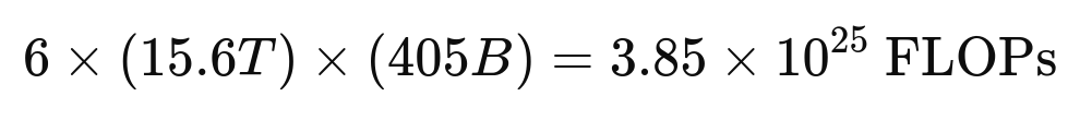Note: this is below the 10²⁶ FLOPs threshold outlined in recent U.S. executive orders, which mandates additional regulatory oversight for AI models exceeding that limit.

Compute Infrastructure

The model was trained on 16,000 H100 GPUs, each delivering an estimated 400 TFLOPS of performance. Given this, the total training time is computed as:

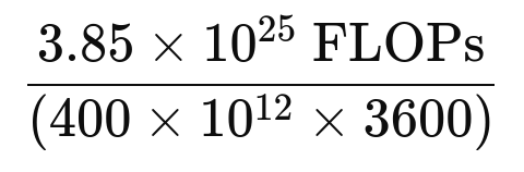
which translates to 26 million GPU hours, or approximately 70 days for completion. Meta reported using 30 million GPU hours, suggesting some inefficiencies or additional redundancy in the training process.

Training Costs

The estimated cost for training LLaMA 3 includes:

• GPU rental: Assuming a lower-bound cost of $2 per GPU hour, this totals to $52 million.
• Employee salaries: With an estimated 50 engineers at an average salary of $500K per year, this adds around $25 million.
• Total cost estimate: $75 million (within a ±$10M margin).

Carbon Footprint

Energy consumption translates to a carbon footprint of ~4,400 tons of CO₂, roughly comparable to 2,000 round-trip flights from New York (JFK) to London (LHR).

Future Scaling Trends

If the current trend continues, each new generation of models will have ~10× more FLOPs. This suggests that future frontier models (e.g., GPT-5 or LLaMA 4) could require 10²⁶ FLOPs, potentially crossing regulatory thresholds and further amplifying compute, cost, and energy demands.

This concludes the overview of pretraining. The second part in the article series will cover post-training or alignment that enabled the development of ChatGPT from GPT-3.