Integrated Gradients: AI Explainability for Regulated Industries

Usage of AI models in highly regulated sectors like finance and healthcare comes with a critical responsibility: explainability. It is not enough that your model predictions are accurate. You should be in a position to explain why your model made a specific prediction. For example, if we are developing a tumor detection model based on brain MRI scans, we should be able to explain what information our model uses and how it processes that information and leads to tumor identification. In this case, regulators or doctors need to know these details to ensure unbiased and accurate results. So, how do you explain your model decision? Explaining them manually is not easy as there's no simple "if-else" logic — deep learning models might often have millions of parameters interacting in non-linear ways, making it impossible to trace the path from input to output. 

One of the techniques that I have had hands-on experience with in addressing this need is Integrated Gradients. It was introduced back in 2017 by researchers at Google, a powerful method that computes attributions by integrating gradients from a baseline to the actual input. In this article, I will walk you through an image classification use case and show you how integrated gradients help us to understand what image pixels are most important in the decision. I will be using the Captum library for calculating attributions and a pre-trained ResNet model to predict images.

Environment Setup

• Python 3.10 or higher is installed.
• Install the necessary packages mentioned below.

pip install captum torch torchvision Matplotlib NumPy PIL

• Download a sample image and name it as image.jpg (you can download any image that you like).

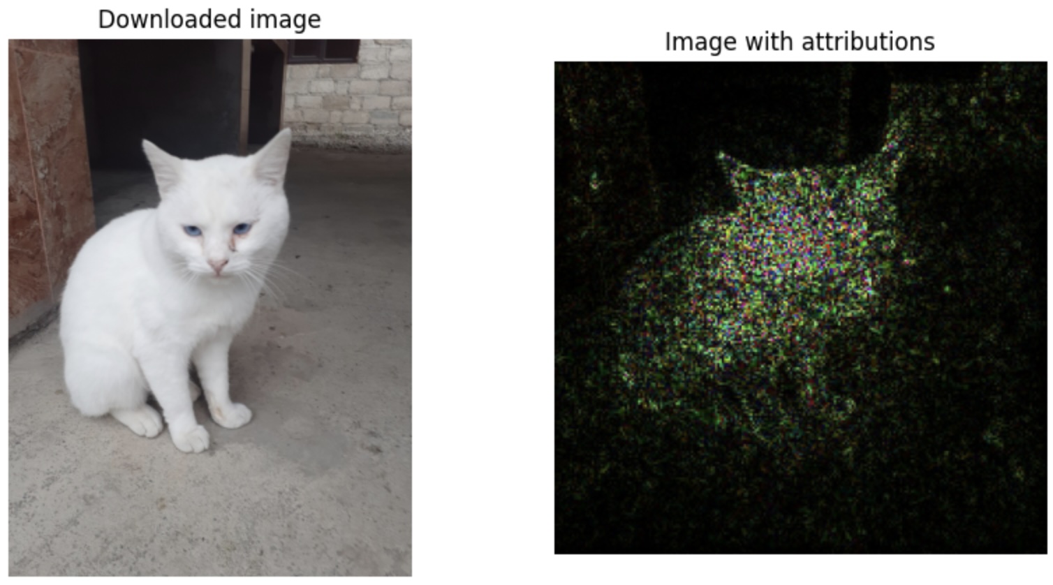
Now, we are going to load the pre-trained ResNet model that knows about the objects, classify the image by using ResNet model, compute attributes using integrated gradients technique and visualize the results that shows which pixels of the image are most important for the model's prediction.

Below is the complete implementation with detailed comments.

import torch
import torchvision
import torchvision.transforms as transforms
from captum.attr import IntegratedGradients
from PIL import Image
import matplotlib.pyplot as plt
import numpy as np

# Load the image that we just downloaded. Change the image name, if you downloaded with different name.
image_to_predicted = Image.open('image.jpg')

# Resize the image into standarad format and convert it into numbers.
transformed_image = transforms.Compose([
    transforms.Resize((224, 224)),
    transforms.ToTensor()
])(image_to_predicted).unsqueeze(0)

# Download pre-trained ResNet model make it ready for prediction.
model = torchvision.models.resnet18(pretrained=True)
model.eval()

# Making the predictio and using argmax function to find the object with the highest probability.
predicted_image_class = torch.nn.functional.softmax(model(transformed_image)[0], dim=0).argmax().item()

# creating IntegratedGradients object and calculate the attributes
integrated_gradiants = IntegratedGradients(model)

# Creating baseline reference from which the IG computation starts
baseline_image = torch.zeros_like(transformed_image)

# compute attributions by using predicted image class, baseline and transformed image
computed_attributions,delta = integrated_gradiants.attribute(transformed_image, baseline_image, target=predicted_image_class, return_convergence_delta=True)

# Convert attributions to numpy array for visualization
attributions_numpy = np.abs(np.transpose(computed_attributions.squeeze().cpu().detach().numpy(), (1, 2, 0))) * 255 * 10
attributions_numpy = attributions_numpy.astype(np.uint8)

# Visualize both downloaded image and image with attributions
fig, axes = plt.subplots(1, 2, figsize=(10, 5))
axes[0].imshow(img)
axes[0].axis('off')
axes[0].set_title('Downloaded image')
axes[1].imshow(attributions_numpy,cmap='magma')
axes[1].axis('off')
axes[1].set_title('Image with attributions')
plt.show()

Here is the output for the sample image that I downloaded. You can see the highlighted area that shows the importance of each pixel for the model's prediction.

Conclusion

In this tutorial, we have explored how Integrated Gradients can be used to explain the predictions of a deep learning model. Using Integrated Gradients, we have gained insights into which pixels of an image are most important for the model's prediction. This is not the only technique available for model explainability. Other techniques like Feature Importance, Shapley Additive Explanations (SHAP) can also be used to gain insights into model behavior.