Kalman Filters With Apache Spark Structured Streaming and Kafka
We discuss Kalman filters and gave an example of how to use them in combination with Apache Spark Structured Streaming and Kafka.
Join the DZone community and get the full member experience.
Join For FreeIntroduction
In simple terms, a Kalman filter is a theoretical model to predict the state of a dynamic system under measurement noise. Originally developed in the 1960s, the Kalman filter has found applications in many different fields of technology including vehicle guidance and control, signal processing, transportation, analysis of economic data, and human health state monitoring, to name a few (see the Kalman filter Wikipedia page for a detailed discussion). A particular application area for the Kalman filter is signal estimation as part of time series analysis. Apache Spark provides a great framework to facilitate time series stream processing. As such, it would be useful to discuss how the Kalman filter can be combined with Apache Spark.
In this article, we will implement a Kalman filter for a simple dynamic model using the Apache Spark Structured Streaming engine and an Apache Kafka data source. We will use Apache Spark version 2.3.1 (latest, as of writing this article), Java version 1.8, and Kafka version 2.0.0. The article is organized as follows: the next section gives an overview of the dynamic model and the corresponding Kalman filter; the following section will discuss the application architecture and the corresponding deployment model, and in that section we will also review the Java code comprising different modules of the application; then, we will show graphically how the Kalman filter performs by comparing the predicted variables to measured variables under random measurement noise; we'll wrap up the article by giving concluding remarks.
The source code for the application discussed in this article can be downloaded from GitHub.
Kalman Filter and Sample Dynamic Models
Kalman filters provide an algorithm to predict variables of a dynamic system under observation where both the system itself and the measurements (observation) are subjected to noise. With proper modeling, many different types of real-time systems can be analyzed using Kalman filters. As an example, the Splunk Enterprise Machine Learning Toolkit has a predict method for time series forecasting based on Kalman filters. That method can be used for a variety of purposes, e.g. sales prediction or forecasting web site access. In a research study, Kalman filters were utilized to predict human body temperature from heart rate using a wearable sensor. Another recent application of Kalman filters is traffic flow prediction using past and real-time observations.
A direct comparison between Kalman filters and machine learning techniques, such as artificial neural networks or binary trees, is difficult to do because of inherent differences. A Kalman filter is based on some prior knowledge of a system in terms of mathematical equations involving inputs to the system, internal dynamics, and how internal dynamics are measured to produce an output. A training phase for a Kalman filter is not required. Furthermore, a Kalman filter operates by consuming real-time output of the actual system under both measurement and process noise. On the other hand, artificial neural networks or binary trees do not require prior knowledge of the system in terms of mathematical equations. However, they require a prior training phase with data that is as accurate as possible. In addition, once the model is trained any ongoing disturbances on the original system (process noise) that could affect its behavior cannot be taken into account.
The following table tries to summarize those observations.
| Kalman Filter | Artificial Neural Network or Binary Tree | |
| Prior knowledge of system model | Required | Not required |
| Training phase | Not required | Required |
| Operation under measurement noise | Filter performs successfully under measurement noise (certain conditions should hold on the randomness of measurement noise) |
In general, training and validation data should be accurate, however, a small amount of faulty data could be tolerated along with sufficiently large accurate data. Once training and validation is done, input to processed by the algorithm must be accurate. |
Operation under process noise |
Filter performs successfully under process noise (certain conditions should hold on the randomness of process noise) |
Once training and validation is done, any external input that could change behavior of the original system cannot be taken into account by the algorithm. |
The dynamic model discussed in this article is a linear system representing the two dimensional motion of an object under measurement noise. The below diagram shows basic elements of the process.
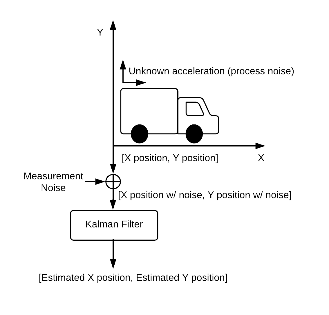 Figure 1. Dynamic system.
The object has unknown acceleration along both X and Y axes (process noise). Position of the object is measured along X and Y axes, however, both measurements are affected by noise. As a result, actual position is not available. The measurements under noise are fed into the Kalman filter that produces an estimated position.
In our sample application, we will use three distinct Amazon EC2 server instances as shown below.
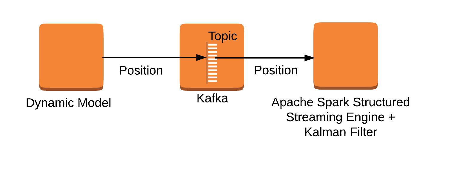
Figure 2. Main components of the application.
One instance will simulate the linear model representing the object's position. Another instance will run a Kafka topic. The position of object will be pushed to the Kafka topic at periodic intervals. The third instance will run the Kalman filter combined with the Spark Structured Streaming engine to consume the system dynamics from the Kafka topic. Here, we will simulate the measurement noise while reading data from Kafka (the application code is written so that, if needed, all three components can be run in the same machine, e.g. a local laptop computer).
Some Theory
We will try to describe the theory around Kalman filters as simply as possible (for interested readers, the Wikipedia page provides more in-depth knowledge). Our coverage of the filter will be limited to the particular dynamic model being discussed in the article and closely follows the lecture notes from Stanford University as well as the lecture notes from the University of Utah.
System Dynamics
Let xk and ẋk be the position and speed along the x axis, respectively, of an object at measurement point k, k being an integer 0, 1, 2, ... Similarly, let yk and ẏk be the position and speed along the y axis, respectively, of the object at measurement point k. Assume that the object has unknown acceleration due to process noise represented by pxk along the x axis and pyk along the y axis, at measurement point k (there is no input to system other than process noise). Then, we call [xk ẋk yk ẏk]Tas a state vector and [pxk pyk]T as a process noise vector of the dynamic system where T represents matrix transposition.
A linear equation for the system can be written as follows:
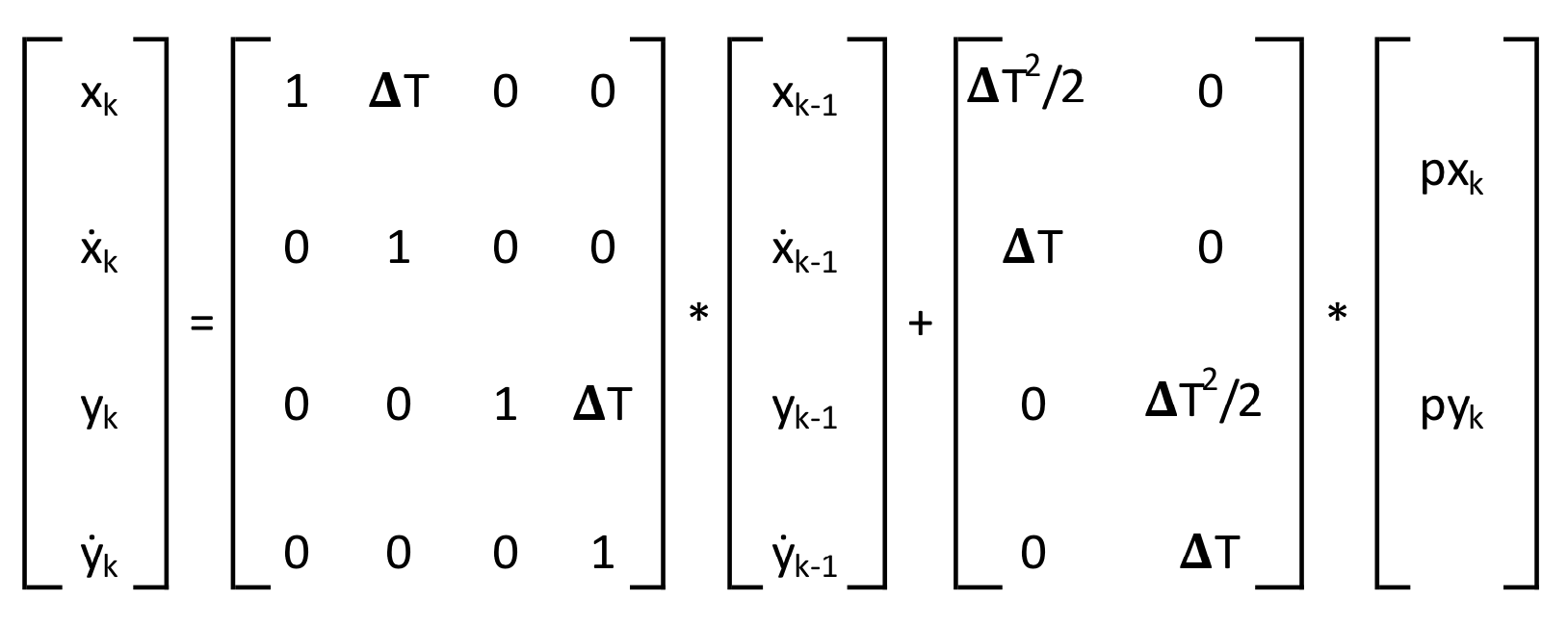
where ΔT is the time interval between measurement points k and k-1. From the equation above, define state matrix F and process input matrix G as
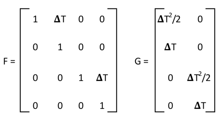
Thus [xk ẋk yk ẏk]T = F * [xk-1 ẋk-1 yk-1 ẏk-1]T + G * [pxk pyk]T .
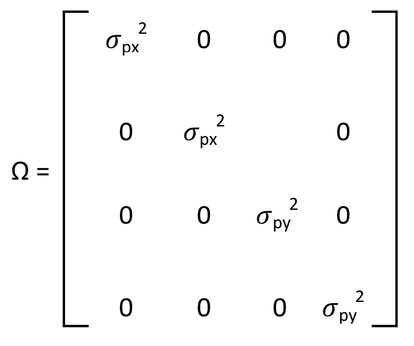
We mentioned that acceleration in either direction, pxk and pyk, results from process noise and is unknown. We make an assumption that both pxk and pyk are independent Gaussian random variables with zero mean and variances σpx2, σpy2, respectively, between measurement points k and k-1. Denote the corresponding covariance matrix by Q, given by Q = Ω * G * GT where Ω is defined as
The information covered so far is all needed for representing the dynamic state of our object.
Measuring the System Dynamics
Let vxk and vyk be the measurement noise affecting xk and yk, respectively, and let mxk and myk be the resulting measurements. More precisely, mxk = xk + vxk and myk = yk + vyk. Define:
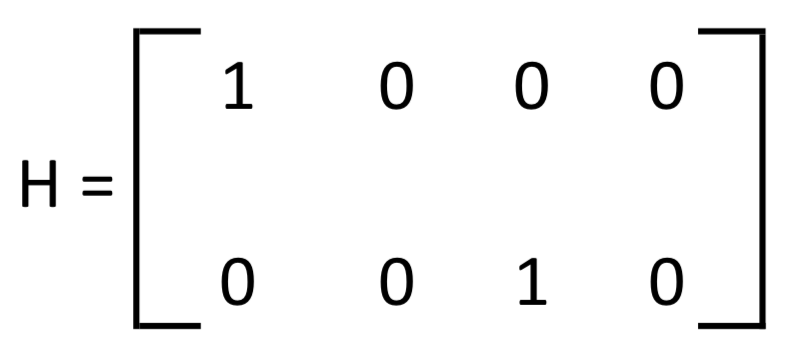
Observe that [mxk myk]T = H * [xk ẋk yk ẏk]T + [vxk vyk]T. Assume that both vxk and vyk are independent Gaussian random variables with zero mean and variances σvx2, σvy2, respectively, between measurement points k and k-1. The corresponding covariance matrix R is defined as:
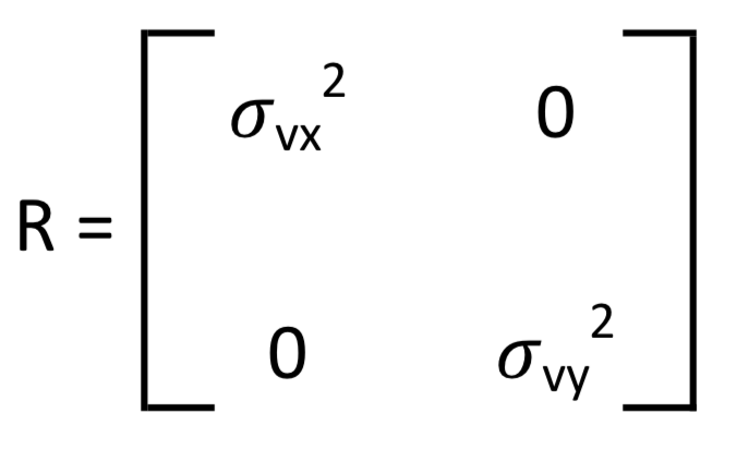
Define vector Xk|k to be the estimate of state vector, [xk ẋk yk ẏk]T. With a Kalman filter, our goal is to generate Xk|k as closely to [xk ẋk yk ẏk]T as possible. We also define Pk|k as the error covariance matrix associated with Xk|k, a measure of how accurate an estimate Xk|k is.
Predict Phase
A Kalman filter is a time-varying function calculated in two phases, a predict phase and an update phase. For the predict phase, we define Xk|k-1 to be the predicted state estimate:
(Eq. 1) Xk|k-1 = F * Xk-1|k-1
Also define Pk|k-1 as the predicted error covariance for Pk|k:
(Eq. 2) Pk|k-1 = F * Pk-1|k-1 * FT+ Q
Update Phase
For the update phase, define an auxiliary vector zk and an auxiliary matrix Sk as follows:
(Eq. 3) zk = [mxk myk]T - H * Xk|k-1
(Eq. 4) Sk = H * Pk|k-1 * HT + R
Then, the so-called optimal Kalman gain Kk is defined as:
(Eq. 5) Kk = Pk|k-1 * HT * Sk-1
Finally,
(Eq. 6) Xk|k = Xk|k-1 + Kk * zk
(Eq. 7) Pk|k = (I - Kk * H) * Pk|k-1
where I denotes the identity matrix.
To recap the discussion above, observe that the computational steps are recursive. At a measurement point k, we utilize Eq. 1, 2 to calculate Xk|k-1 and Pk|k-1 from knowledge of Xk-1|k-1 and Pk-1|k-1. That completes the predict phase. Then, following Eq. 3, 4 we calculate the auxiliary vector zk and the auxiliary matrix Sk. (Observe that measurement is incorporated in Eq. 3.) Afterwards, we utilize Eq. 5 to compute the optimal Kalman gain Kk. Finally, we use Eq. 6, 7 to obtain Xk|k and Pk|k. Hence, starting with Xk-1|k-1 and Pk-1|k-1, we end up obtaining Xk|k and Pk|k at each iteration.
It should be noted that at closely initial measurement point k = 0 we need P0|0 and an estimate X0|0 of [x0 ẋ0 y0 ẏ0]T for the recursion to start. Typically, P0|0 is guessed. If closely initial value of the state vector is known, X0|0 is set to it. Otherwise, X0|0 is also guessed.
Code Review
We have two separate modules, State-Model and the Kalman-Filter written in Java. The State-Model implements the dynamic model and generates state vector elements xk, ẋk, yk and ẏk. The Kalman-Filter implements the Kalman filter and generates Xk|k. Referring to Fig. 2, the State-Model is deployed into the server instance with label 'Dynamic Model' whereas the Kalman-Filter is deployed into the server instance with the label 'Apache Spark Structured Streaming Engine + Kalman Filter.' The Java package and class structure is as follows.
State-Model:
org.demo.spark.streaming.UtilsAndConstants
org.demo.spark.streaming.producer.TopicWriter
org.demo.spark.streaming.producer.StateModel
Kalman-Filter:
org.demo.spark.streaming.UtilsAndConstants
org.demo.spark.streaming.consumer.KalmanFilter
UtilsAndConstants.java
This class provides various matrix operations based on the org.apache.spark.ml.linalg library. In addition, it includes constants used by both the State-Model and the Kalman-Filter modules. It is shared by the State-Model and the Kalman-Filter.
package org.demo.spark.streaming;
import org.apache.spark.ml.linalg.DenseMatrix;
import org.apache.spark.ml.linalg.DenseVector;
import org.apache.spark.ml.linalg.Matrix;
import org.apache.spark.ml.linalg.Vector;

public class UtilsAndConstants {
  public static final String SEPARATOR = "^";
  public static final String SEPARATOR_RGX = "\\^";

  public static final double DT = 0.01;
  public static final double SIGMA_px = 5;
  public static final double SIGMA_py = 4;

  public static DenseMatrix G;
  static {
    double vals[] = {Math.pow(UtilsAndConstants.DT,2)/2,
                     UtilsAndConstants.DT,0,0,0,0,
                     Math.pow(UtilsAndConstants.DT,2)/2,UtilsAndConstants.DT};

    G = new DenseMatrix(4,2, vals);
  }

  public static DenseMatrix F;
  static {
    double[] vals = {1,0,0,0,UtilsAndConstants.DT,1,0,0,0,0,
                     1,0,0,0,UtilsAndConstants.DT,1};
    F = new DenseMatrix(4,4,vals);
  }
  ...
The SEPARATOR and SEPARATOR_RGX will be used when state dynamics are transferred through Kafka as we will review later on. The scalar constants DT, SIGMA_px, SIGMA_py and matrix constants G, F correspond to ΔT, σpx, σpy, G, F introduced earlier. Note that G and F are of type org.apache.spark.ml.linalg.DenseMatrix. We assume that unit of time for DT is second, i.e. DT represents 0.01 second.
The following method calculates the inverse of a matrix based on an external library, Jama Java Matrix Package.
public static DenseMatrix inverse(DenseMatrix input){
  int size = input.numCols();
  return new DenseMatrix(size,size,
     ((new Jama.Matrix(input.values(),size)).inverse()).getColumnPackedCopy());
}
...
The org.apache.spark.ml.linalg library currently does not provide a method for matrix inversion and that is why we chose to employ an external library. It should be noted that the org.apache.spark.mllib.linalg library provides singular value decomposition that can be used for matrix inversion. However, Apache Spark is currently transitioning to DataFrame-based APIs, mainly supported by the org.apache.spark.ml.linalg package whereas the org.apache.spark.mllib.linalg package is oriented towards RDD-based APIs (see the discussion here). In this article, we did not want to mix and match org.apache.spark.ml.linalg (our main focus) with org.apache.spark.mllib.linalg and therefore our workaround was to use Jama Java Matrix Package for matrix inversion.
The following method adds or subtracts two org.apache.spark.ml.linalg.Vector instances to return an org.apache.spark.ml.linalg.DenseVector.
public static DenseVector addOrSubtract(Vector a, Vector b, boolean isAdd){
  double[] tmp1 = a.toArray();
  double[] tmp2 = b.toArray();
  double[] tmp3 = new double[tmp1.length];
  int factor = 1;
  if(!isAdd){
    factor = -1;
  }
  for(int i = 0; i < tmp1.length; i++){
    tmp3[i] = tmp1[i] + factor*tmp2[i];
  }
  return new DenseVector(tmp3);
}
...
The following method multiples every element of a DenseMatrix with a scalar and returns the newly constructed matrix.
public static DenseMatrix scale(DenseMatrix input, double factor){
  double[] vals = input.toArray();
  double[] newVals = new double[vals.length];
  for(int i = 0; i < vals.length; i++){
    newVals[i] = factor * vals[i];
  }
  return new DenseMatrix(input.numRows(), input.numCols(), newVals);
}
The following method creates a String object from the elements of an org.apache.spark.ml.linalg.Vector instance separated with "^".
public static String formatElements(Vector vector){
  double[] tmp = vector.toArray();
  StringBuilder bldr = new StringBuilder();
  for(int i = 0; i < tmp.length; i++){
    bldr.append(tmp[i]).append(SEPARATOR);
  }
  String tmpStr = bldr.toString();
  return (tmpStr).substring(0,tmpStr.length() - 1);
}
The following is the last method in UtilsAndConstants to review. It adds two org.apache.spark.ml.linalg.Matrix instances to return an org.apache.spark.ml.linalg.DenseMatrix.
public static DenseMatrix add(Matrix a, Matrix b) throws RuntimeException{
  if(a.numRows() != b.numRows() || a.numCols() != b.numCols()){
    throw new
      RuntimeException
      ("Matrices with incompatible dimensions cannot be added!");
  }
  double[] tmp1 = a.toArray();
  double[] tmp2 = b.toArray();
  double[] tmp3 = new double[tmp1.length];
  for(int i = 0; i < tmp1.length; i++){
    tmp3[i] = tmp1[i] + tmp2[i];
  }
  return new DenseMatrix(a.numRows(),a.numCols(),tmp3);
}
TopicWriter.java
This class encapsulates the logic writing into a Kafka topic. It closely follows a previously published tutorial.
The class has a static member of type org.apache.kafka.clients.producer.Producer. It also has topic and server instance names, TOPIC_NAME and SERVER_NAME.
package org.demo.spark.streaming.producer;

import org.apache.kafka.clients.producer.Producer;
import org.apache.kafka.clients.producer.ProducerRecord;
import org.apache.kafka.clients.producer.ProducerConfig;
import org.apache.kafka.clients.producer.KafkaProducer;
import org.apache.kafka.common.serialization.LongSerializer;
import org.apache.kafka.common.serialization.StringSerializer;
import java.util.Properties;

public class TopicWriter {
  private static Producer<Long, String> producer = null;
  private static String TOPIC_NAME = null;
  private static String SERVER_NAME = null;
  ...
The init() method sets values for TOPIC_NAME and SERVER_NAME.
public static void init(String bootstrapServer, String topic) {
  SERVER_NAME = bootstrapServer;
  TOPIC_NAME = topic;
}
...
The following method initializes the org.apache.kafka.clients.producer.Producer instance and returns it.
private static Producer<Long, String> getProducer() {
  Properties properties = new Properties();
  properties.put(ProducerConfig.BOOTSTRAP_SERVERS_CONFIG,
                 SERVER_NAME);
  properties.put(ProducerConfig.CLIENT_ID_CONFIG, "TopicWriter");
  properties.put(ProducerConfig.KEY_SERIALIZER_CLASS_CONFIG,
                 LongSerializer.class.getName());
  properties.put(ProducerConfig.VALUE_SERIALIZER_CLASS_CONFIG,
                 StringSerializer.class.getName());
  return new KafkaProducer<>(properties);
}
...
Below is the method to write into the topic using the Producer.
public static void write(String message){
  if(producer == null){
    producer = getProducer();
  }    long time = System.currentTimeMillis();
  final ProducerRecord<Long, String> record =
    new ProducerRecord<>(TOPIC_NAME, time,  message);
  producer.send(record);
  producer.flush();
}
...
Finally, close the Producer instance using the close( method below.
    public static void close(){
      if(producer == null){
        producer.close();
      }
    }
}
StateModel.java
This class implements the dynamic system. We start with initializing several variables. PROCESS_NOISE_X and PROCESS_NOISE_Y are Random variables used to describe the process noise. The F and G are the local copies of the state and process input matrices already defined in UtilsAndConstants. The vector X_a_current represents the state vector of the system. We pick arbitrary values to initialize X_a_current.
package org.demo.spark.streaming.producer;

import org.apache.log4j.Level;
import org.apache.log4j.Logger;
import org.apache.spark.ml.linalg.DenseMatrix;
import org.apache.spark.ml.linalg.DenseVector;
import org.apache.spark.ml.linalg.Vector;
import org.demo.spark.streaming.UtilsAndConstants;
import java.util.Random;

public class StateModel {
  private static Random PROCESS_NOISE_X = new Random(23423874764L);
  private static Random PROCESS_NOISE_Y = new Random(96653878224L);
  private static DenseMatrix F = UtilsAndConstants.F;
  private static DenseMatrix G = UtilsAndConstants.G;

  private static Vector X_a_current;
  static {
    double[] vals = {0,5,3,1}; // position x, speed x, position y, speed y
    X_a_current = new DenseVector(vals);
  }
  ...
The following method updates the state vector from previous state and process noise. The variables p_x and p_y correspond to pxk and pyk at measurement point k. The last line simply emulates the equation
[xk ẋk yk ẏk]T = F * [xk-1 ẋk-1 yk-1 ẏk-1]T + G * [pxk pyk]T
private static void updateXa(){
  double p_x = PROCESS_NOISE_X.nextGaussian() * UtilsAndConstants.SIGMA_px;
  double p_y = PROCESS_NOISE_Y.nextGaussian() * UtilsAndConstants.SIGMA_py;

  double[] vals = {p_x,p_y};
  DenseVector processNoise = new DenseVector(vals);
  X_a_current = UtilsAndConstants.addOrSubtract(F.multiply(X_a_current),
      G.multiply(processNoise), true);
}
...
Our main method listed below is very simple. At startup, names should be given to the Kafka bootstrap server and a topic name should be supplied, otherwise an error condition occurs. After checking the validity of the startup parameters, we initialize the Kafka producer via TopicWriter.init() and let the dynamic system run 1,500 iterations (because DT is 0.01 second, this is a 15 second simulation). At each iteration, the state vector is calculated and its elements are written into the Kafka topic. We finally close the Kafka producer via TopicWriter.close().
    public static void main(String[] args){
      if (args.length < 2) {
        System.err.println("Usage: StateModel <bootstrap-server> <topic>");
        System.exit(1);
      }
      Logger.getRootLogger().setLevel(Level.FATAL);
      TopicWriter.init(args[0],args[1]);
      for(int i = 0; i < 1500; i++){
        TopicWriter.write(UtilsAndConstants.formatElements(X_a_current));
        updateXa();
      }
      TopicWriter.close();
    }
}
KalmanFilter.java
This method implements the Kalman filter. We start with defining various constants. SUBSCRIBE is the subscription type for Kafka topic. OBSERVATION_NOISE_x and OBSERVATION_NOISE_y will be used to generate noise variables vxk and vyk. The SIGMA_px, SIGMA_py are the local copies of the same variables defined in UtilsAndConstants.
package org.demo.spark.streaming.consumer;

import org.apache.log4j.Level;
import org.apache.log4j.Logger;
import org.apache.spark.ml.linalg.DenseMatrix;
import org.apache.spark.ml.linalg.DenseVector;
import org.apache.spark.ml.linalg.Matrix;
import org.apache.spark.ml.linalg.Vector;
import org.apache.spark.sql.SparkSession;
import org.apache.spark.sql.streaming.StreamingQuery;
import org.apache.spark.sql.Dataset;
import org.apache.spark.sql.Encoders;
import org.apache.spark.sql.ForeachWriter;
import org.demo.spark.streaming.UtilsAndConstants;
import java.util.Random;

public class KalmanFilter {
  private static String SUBSCRIBE = "subscribe";
  private static Random OBSERVATION_NOISE_x = new Random(17686267572368l);
  private static Random OBSERVATION_NOISE_y = new Random(40639867672371l);
  private static final double SIGMA_px = UtilsAndConstants.SIGMA_px;
  private static final double SIGMA_py = UtilsAndConstants.SIGMA_py;
  ...
Next, we define the local copies of matrices G and F and define F_T, transpose of F.
private static DenseMatrix G = UtilsAndConstants.G;
private static DenseMatrix F = UtilsAndConstants.F;
private static DenseMatrix F_T = F.transpose();
...
This is followed by definitions of matrices R, Q, H and H_T, transpose of H.
private static Matrix R;
static {
  double[] vals = {Math.pow(SIGMA_px,2),0, 0,Math.pow(SIGMA_py,2)};
  R =  new DenseMatrix(2,2,vals);
}

private static Matrix Q;
static {
  double[] vals = {Math.pow(SIGMA_px,2), 0, 0, 0,
                   0, Math.pow(SIGMA_px,2), 0, 0,
                   0, 0, Math.pow(SIGMA_py,2), 0,
                   0, 0, 0, Math.pow(SIGMA_py,2)};

  Q = (new DenseMatrix(4,4,vals)).multiply(G).multiply(G.transpose());
}

private static DenseMatrix H;
static {
  double[] vals = {1,0, 0,0, 0,1, 0,0};
  H = new DenseMatrix(2, 4,vals);
}

private static DenseMatrix H_T = H.transpose();
...
Then, we define P_current and X_current to represent Pk|k and Xk|k, respectively. It was previously mentioned that we need initial values P0|0 and X0|0. We arbitrarily choose P0|0 as an all zero matrix and X0|0 = [4 0 0 0]T.
private static DenseMatrix P_current;
static {
  P_current = UtilsAndConstants.scale(DenseMatrix.eye(4),0);
}

private static Vector X_current;

static {
  double[] vals = {4,0,0,0};
  X_current = new DenseVector(vals);
};
...
For the predict phase, the following methods implement Eq. 1, 2, respectively. Hence getNextX() returns the predicted state estimate and getNextP() returns the predicted error covariance for Pk|k.
private static Vector getNextX(){
  return F.multiply(X_current);
}

private static DenseMatrix getNextP(){
  DenseMatrix nextP = UtilsAndConstants.add(F.multiply(P_current)
                                            .multiply(F_T),Q);
  return nextP;
}
...
In preparation of the update phase, the following method generates observation noise.
private static DenseVector getObservationNoiseVector(){
  double dx = OBSERVATION_NOISE_x.nextGaussian() * SIGMA_px;
  double dy = OBSERVATION_NOISE_y.nextGaussian() * SIGMA_py;
  double[] d = new double[2];
  d[0] = dx;
  d[1] = dy;
  return new DenseVector(d);
}
...
Then, in update phase, the following methods implement Eq. 3 - 5.
private static DenseVector getZ(DenseVector y){
  return UtilsAndConstants.addOrSubtract(y, H.multiply(getNextX()),false);
}

private static DenseMatrix getS(){
  return UtilsAndConstants.add((H.multiply(getNextP())).multiply(H_T), R);
}

private static Matrix getK(){
  return getNextP().multiply(H_T).multiply(UtilsAndConstants.inverse(getS()));
}
...
Then, the below method implements Eq. 6, 7 (variables P_current and X_current).
private static void updateXandP(DenseVector y){
  DenseVector z = getZ(y);
  Matrix K = getK();
  P_current = UtilsAndConstants.add(DenseMatrix.eye(4),
     UtilsAndConstants.scale(K.multiply(H),-1)).multiply(getNextP());
  X_current = UtilsAndConstants.addOrSubtract(getNextX(), K.multiply(z), true);
}
...
Finally, let us review the main method that combines all the pieces together. Two startup parameters are needed, the name of the bootstrap Kafka server and the topic name.
public static void main(String[] args) throws Exception {
  if (args.length < 2) {
    System.err.println("Usage: KalmanFilter <bootstrap-server> " +
                       "<topic>");
    System.exit(1);
  }
  Logger.getRootLogger().setLevel(Level.FATAL);
  String bootstrapServer = args[0];
  String topic = args[1];
  ...
If the sanity check on the startup parameters is passed, we initialize the SparkSession and obtain a Dataset from Kafka that represents the stream of lines obtained from Kafka topic. Each line will correspond to a specific state vector written by StateModel as reviewed above.
SparkSession spark = SparkSession
.builder()
  .appName("KalmanFilter").master("local[*]")
  .getOrCreate();

Dataset<String> lines = spark
.readStream()
  .format("kafka")
  .option("kafka.bootstrap.servers", bootstrapServer)
  .option(SUBSCRIBE, topic)
  .load()
  .selectExpr("CAST(value AS STRING)")
  .as(Encoders.STRING());
...
Then we start processing the lines read via the following:
StreamingQuery query = lines.writeStream()
  .foreach(new ForeachWriter<String>() {
  public boolean open(long partitionId, long version) {
    return true;
  }

  public void process(String value) {
    ...
  }

  public void close(Throwable errorOrNull) {}
}).start();
The open() method opens the connection and close() performs cleanup. Let us review the process() method in more detail. It starts with parsing out the line that is just read. From the review of StateModel.java, recall that the line gives the current value of the state vector, i.e. actual values of the state. Then, we extract estimated values from Vector X_current. We continue by obtaining the observation vector [mxk myk]T . We then print out estimated, actual, and observed variables. Finally, we obtain Xk|k and Pk|k via updateXandP()to complete the update phase. That ends the process() method.
public void process(String value) {
   // Actual
   String[] tokens = value.split(UtilsAndConstants.SEPARATOR_RGX);
   String actual_position_x = tokens[0];
   String actual_speed_x = tokens[1];
   String actual_position_y = tokens[2];
   String actual_speed_y = tokens[3];

   double[] vals = {
     Double.parseDouble(actual_position_x),
     Double.parseDouble(actual_speed_x),
     Double.parseDouble(actual_position_y),
     Double.parseDouble(actual_speed_y)
   };

   Vector actual = new DenseVector(vals);

   // Estimated
   double estimated_position_x = (X_current.toArray())[0];
   double estimated_speed_x = (X_current.toArray())[1];
   double estimated_position_y = (X_current.toArray())[2];
   double estimated_speed_y = (X_current.toArray())[3];

   // Observed
   DenseVector observationNoise = getObservationNoiseVector();
   DenseVector observation = UtilsAndConstants.
     addOrSubtract(H.multiply(actual),observationNoise,true);

   double observed_position_x = (observation.toArray())[0];
   double observed_position_y = (observation.toArray())[1];

   System.out.println(estimated_position_x+"|"+observed_position_x+
      "|"+actual_position_x+"|"+estimated_position_y+
      "|"+observed_position_y+"|"+actual_position_y+
      "|"+estimated_speed_x+"|"+actual_speed_x+
      "|"+estimated_speed_y+"|"+actual_speed_y);

   updateXandP(observation);
}
The main() ends as follows.
public static void main(String[] args) throws Exception {
  ...
   query.awaitTermination();
}
Deploying Modules
Creating a Kafka Topic
In the Amazon EC2 instance where we run Zookeeper and Kafka (see figure 2), a one-time configuration needs to be made to create the topic through which State_Model and Kalman_Filter are linked. In that instance, we have Kafka installed in /opt/Kafka/kafka_2.12-1.1.1 folder. First start Zookeeper:
/opt/Kafka/kafka_2.12-1.1.1/bin/zookeeper-server-start.sh \
/opt/Kafka/kafka_2.12-1.1.1/config/zookeeper.properties
Then, start Kafka:
/opt/Kafka/kafka_2.12-1.1.1/bin/kafka-server-start.sh \
/opt/Kafka/kafka_2.12-1.1.1/config/server.properties
Then, execute:
sh bin/kafka-topics.sh --create --zookeeper localhost:2181 \
--replication-factor 1  --partitions 1 --topic testTopic
All commands were executed as root.
Running the Modules
Obtain the source code from GitHub and generate kalman_filter.jar, state_model.jar as described in the README file. Copy each module to the respective Amazon EC2 instance, under the /home/ubuntu folder.
Step 1: In Amazon the EC2 instance where Zookeeper and Kafka are being run, start Zookeeper first and then Kafka as described in the previous section.
Step 2: In the Amazon EC2 instance where kalman_filter.jar is copied, proceed to the folder where the jar file resides and execute:
where <server name> refers to the Amazon EC2 instance where Zookeeper and Kafka are running and <server port> references the Kafka listening port, e.g. 9092.
java -Xmx480m -jar kalman_filter.jar <server name>:<server port> testTopicStep 3: In the Amazon EC2 instance where kalman_filter.jar is copied, proceed to the folder where the jar file resides and execute:
java -Xmx480m -jar state_model.jar <server name>:<server port> testTopicWhen running Step 3, if you observe the console where kalman_filter.jar is running (Step 2), you should see a print out generated by the process() method of KalmanFilter.java, which will look as follows:
...
61.92155575279128|56.80439464693517|60.48344907817928|14.83910569924411|16.287655089759628|15.528272133208104|3.0989093882465717|1.9098255066890608|1.1524546148845474|1.8144043971597563
61.8802515547841|65.41654990335283|60.50304632741667|14.870809776388718|11.936764448564018|15.546334992687862|3.0477906307172304|2.0096243407884726|1.166723608937314|1.7981674987921061
61.95996021208476|61.00326936923335|60.522978878917925|14.841111619092775|16.684959194712405|15.564518246974853|3.0826018110796194|1.9768859594623092|1.1374740415259215|1.8384833586058942
Review of Results
Figures 3 and 4 show the position of the object along X and Y axes, respectively, as a function of time. In both figures, the yellow points denote the measured position with noise, green points show the actual position, and red points show the estimated position after Kalman filter is applied.
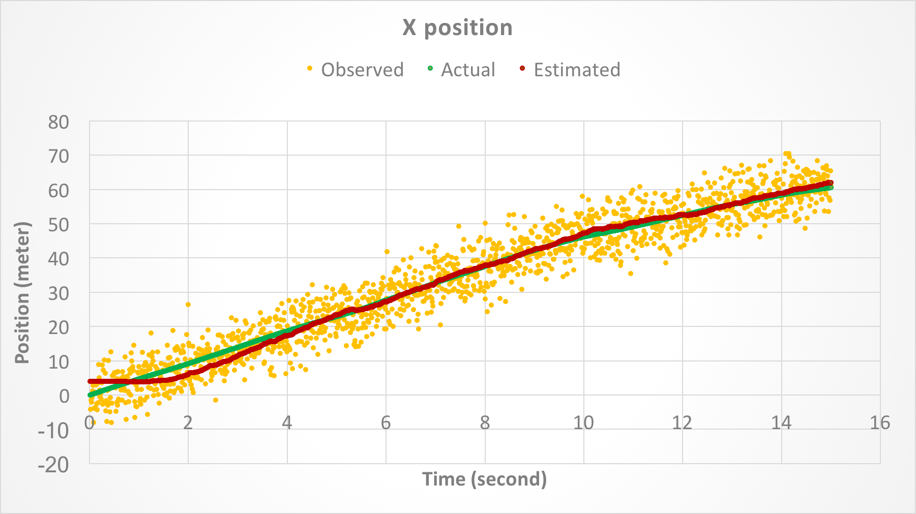
Figure 3. Position of the object along X-axis as a function of time.
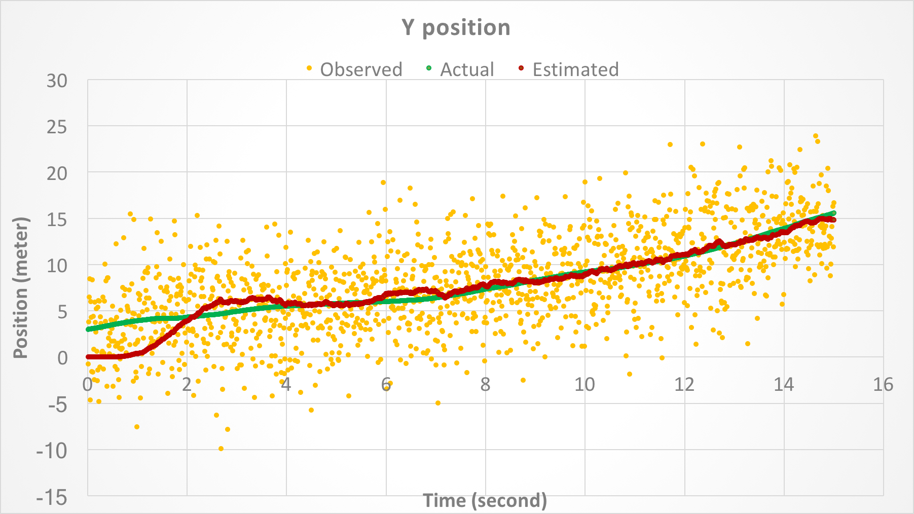
Figure 4. Position of the object along Y-axis as a function of time.
Figures 5 and 6 show the speed of the object along X and Y axes, respectively, as a function of time. In both figures, the green points show the actual speed and the red points show the estimated speed after the Kalman filter is applied. There are no yellow points because speed was not measured.
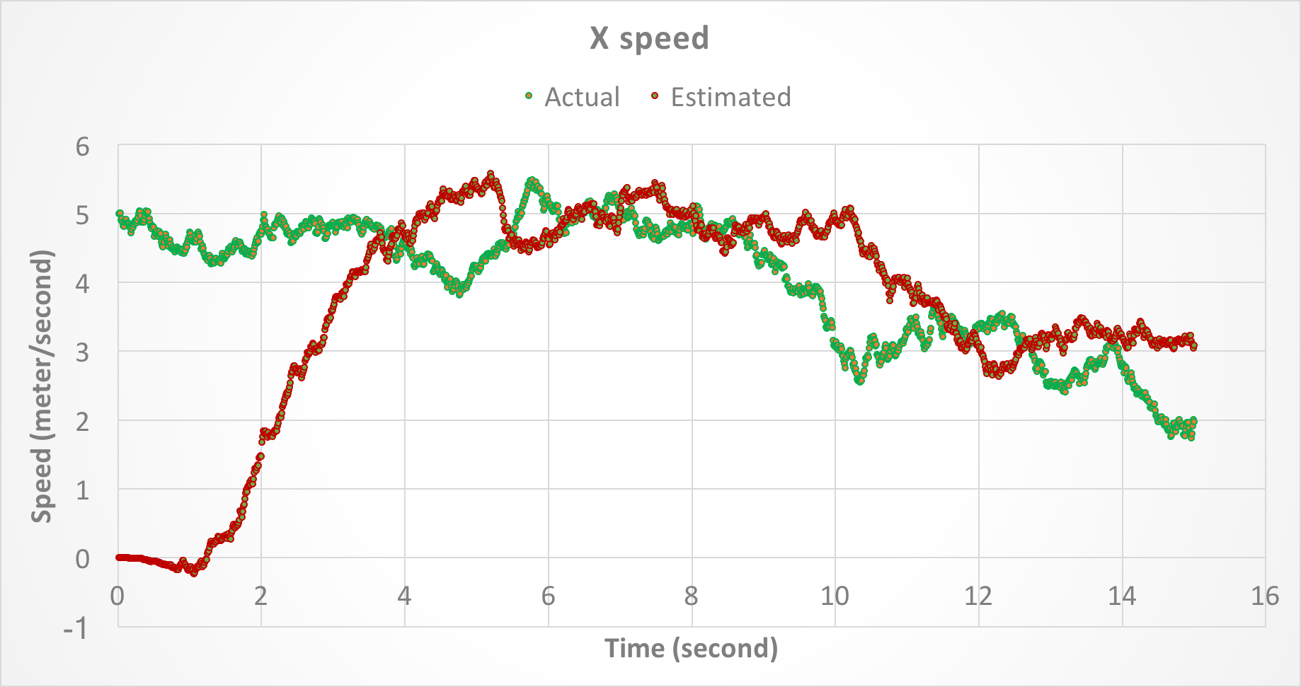
Figure 5. Speed of the object along X-axis as a function of time.
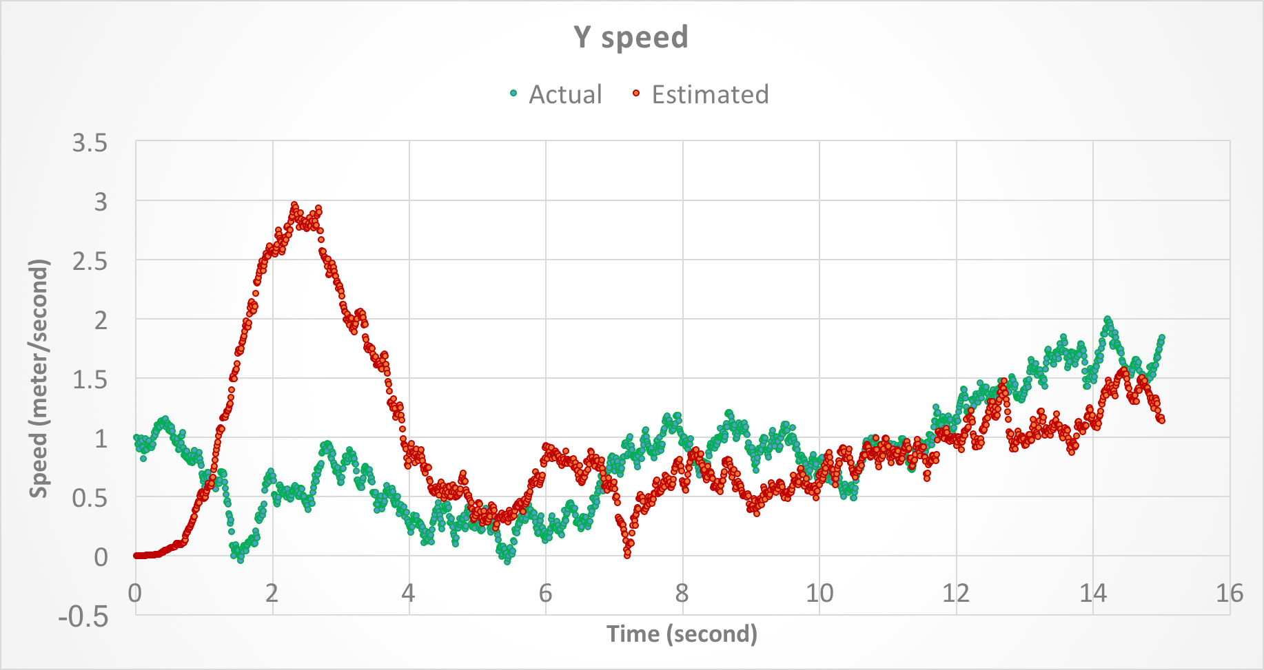
Figure 6. Speed of the object along Y-axis as a function of time.
Finally, the following figure shows position of the object along X and Y axes, combined. Similar to above, the yellow points denote the measured position with noise, green points show the actual position, and red points show the estimated position after the Kalman filter is applied.
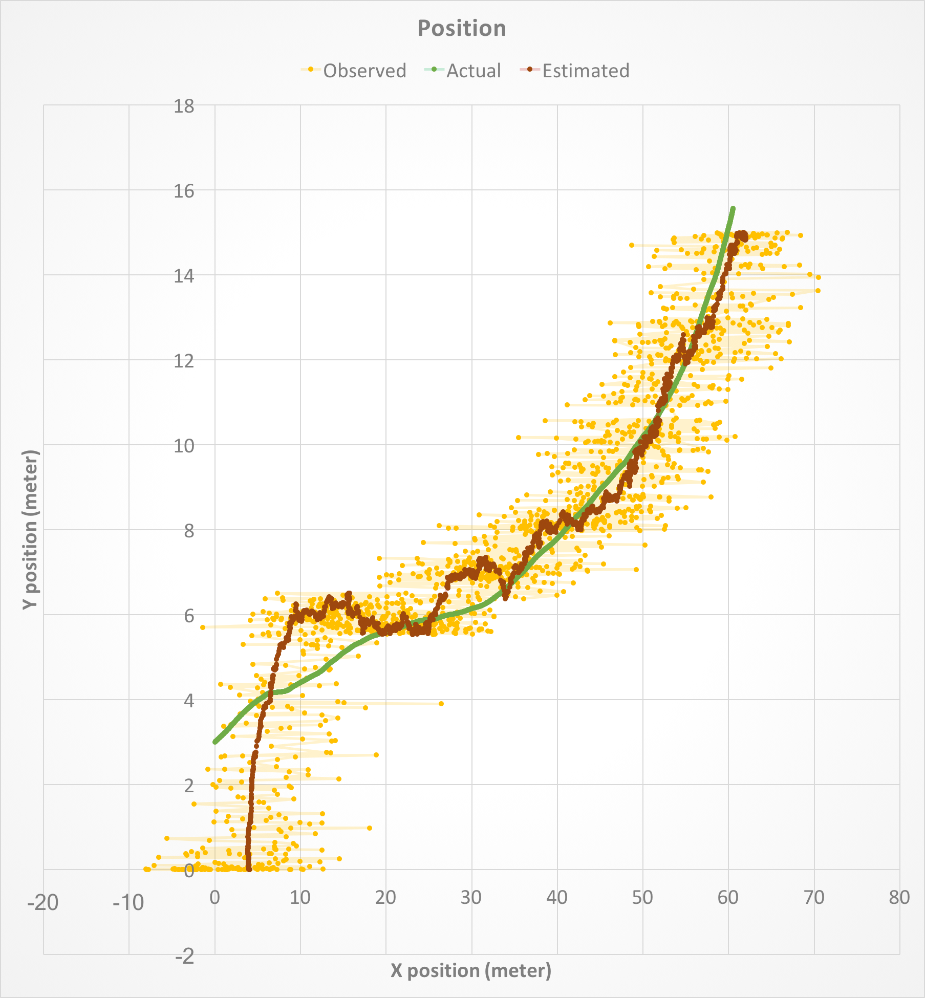
Figure 7. Position of the object along X and Y axes.
Figures 3 - 7 show that the Kalman filter successfully attenuates the noise and is able to track the actual state variables relatively closely. Because the initial state is not known, there is a gap between the estimated and actual state variables at startup. However, the gap is eventually closed as the Kalman filter converges (see also the next section).
Conclusions
In this article, we discussed Kalman filters and gave an example of how to use them in combination with Apache Spark Structured Streaming and Kafka. For a linear, dynamic system with unknown input (process noise) it is shown that the Kalman filter can successfully estimate state variables from noisy measurements.
- Under certain conditions as described in these lecture notes, the Sk and Kk in Eq. 4, 5 will converge to some finite matrices (avoiding a theoretical proof, we assure that the example discussed in the article satisfies those conditions and hence our filter will eventually converge).
- The simple example discussed in the article was concerned with a system with relatively small dimensions. A realistic production environment could involve a system with larger dimensions where matrix operations may cause performance challenges. Keep in mind that performance considerations for matrix operations in Apache Spark currently constitute an active area of research. For example see this article and the one here.
- Extended Kalman filter is an advanced version that deals with nonlinear systems (as opposed to a linear system as discussed in this article). For example, a recent study describes how GPS receiver positioning can be estimated using an extended Kalman filter.
Opinions expressed by DZone contributors are their own.

Comments