

Key ML Classification Metrics You Need to Understand
Accuracy fails on imbalanced data. Learn how Precision, Recall, F1, ROC-AUC, PR-AUC, and Log Loss reveal true classifier performance when error costs diverge.
Accuracy is what many beginners look for when building an ML model. Imagine you have a model that detects skin diseases. Your test dataset has 10,000 patients, out of which only 100 have the disease, while the remaining are healthy. The model ends up predicting everyone as healthy. That would give a 99% accuracy, which sounds impressive, but it failed to identify a single sick patient.
Now, think about deploying it in the real world while blindly trusting its accuracy. That would be disastrous, as it failed to identify even a single sick person during testing. This is why models can fail in the real world even though they gave impressive accuracy during the test phase. To actually understand the model’s behaviour in real life, we need to look at metrics beyond accuracy.
The Confusion Matrix
Let’s start by looking at the confusion matrix, as every binary classification problem falls into one of the four categories. It shows what your model got right and wrong.
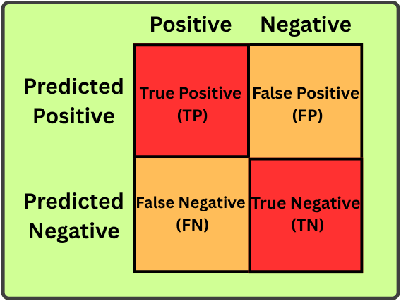
- True Positive (TP): The model predicts that a patient has the disease, and the patient actually has it. The model predicts positive, and it is right.
- True Negative (TN): The model predicts that a patient is healthy, and the patient actually is healthy. The model predicts negative, and it is negative.
- False Positive (FP): The model predicts that a healthy patient has the disease. The model predicts positive, but the actual class is negative.
- False Negative (FN): The model predicts a sick patient as healthy. The model predicts negative, but the actual class is positive.
Before proceeding, make sure you understand all four categories, as they form the foundation for the classification metrics we’ll discuss.
1. Accuracy
Let’s start with the metrics everyone knows. Accuracy measures the percentage of correct predictions out of all predictions made by a model. It is mathematically measured using the formula given below.

Accuracy depends on the training data. In our disease example, we saw that the model failed to detect even a single sick person. This is because the training data must have contained mostly data from healthy people, while only a very small fraction came from sick patients. As a result, it learns that guessing healthy is almost always the safest option and ends up predicting everything as healthy. This is a case of false negatives.
To reduce false negatives, make sure the training data is properly balanced (having equal data for both classes, or adjusting class weights to penalize missing a sick patient). This forces the model to learn the underlying patterns in the data rather than relying on shortcuts.
When to Use Accuracy?
Accuracy works well when:
- The classes are balanced.
- The dataset reflects the real-world class distribution.
- The dataset is balanced, and a false alarm costs the same as missing a detection.
If you are classifying images of dogs and cats and your dataset contains an equal number of both, then accuracy is a great metric. But if classes are imbalanced, then don’t let accuracy fool you.
2. Precision
Many of us are confused between the concepts of accuracy and precision. Accuracy tells how often the model is correct, whereas precision tells how trustworthy the positive predictions are. The mathematical formula for precision is:
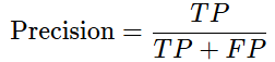
Suppose your model predicts 100 people as sick. But after investigation, it was found that only 70 out of the 100 were sick. That would give a precision score of 70%, which means that 7 out of 10 people predicted as sick are actually sick. A model with low precision is bound to generate false positives.
When to Use Precision?
High precision is needed when:
- False positives can be costly.
- In the case of a spam filter, if a model wrongly classifies a legitimate email as spam, the user might miss an important message.
- If you want a model where a positive prediction is highly likely to be actually positive, you need high precision.
3. Recall
Out of all the actual positive cases, how many accurate predictions does the model make? That's what recall measures. Imagine a model is testing 100 people who are actually sick. If the model correctly identifies 90 of them as sick, then its recall is 90%. The mathematical formula for recall is:
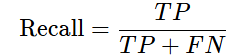
In simple terms, recall tells us how well a model finds the positive cases that are actually there. Recall decreases when the model misses actual positive cases.
When to Use Recall?
Recall is used when:
- Missing a positive case is costly.
- Cases like medical screening where failing to detect a sick person can be deadly.
- Fraud detection, security setups, and search systems.
4. F1-Score
Imagine you are training a fraud detection model to be more aggressive so its recall increases. But an overly aggressive model can sometimes flag a legitimate transaction as fraud, resulting in an increased recall but decreased precision. To avoid imbalance between precision and recall, we can use a metric called F1-Score.

F1-Score is the harmonic mean of both precision and recall. We use the harmonic mean over the arithmetic mean because the harmonic mean heavily penalizes situations where one value is much lower than the other. For example, if we consider a precision of 0.90 and a recall of 0.10, the arithmetic mean would give a result of 0.50, whereas the harmonic mean would yield 0.18.
The value 0.18 gives a better idea that the model is performing poorly on one side of the problem.
When to Use F1-Score?
F1-Score is useful when:
- The classes are imbalanced.
- Both precision and recall matter.
- A single metric that represents both.
However, don’t always use F1-Score just because the classes are imbalanced. You should consider the type of error that matters most in your use case and choose the metrics accordingly.
5. ROC-AUC
A classification model produces a probability score before prediction and uses a threshold to determine whether to classify the input as positive or negative. Consider a threshold of 0.5; any score greater than or equal to 0.5 is considered positive, whereas less than that is negative. A fixed threshold is not always suitable for every problem. Lowering the threshold helps the model find more positive cases, but it can also lead to more false alarms. Raising the threshold reduces false alarms, but the model may miss some of the actual positive cases.
So instead of evaluating the model at just one cutoff, we can use a metric called ROC-AUC, which evaluates its performance across every possible threshold from 0 to 1. The ROC then plots two values: true positive rate (TPR/recall) on the y-axis and false positive rate (FPR) on the x-axis. These values are plotted across different thresholds to form the ROC curve.
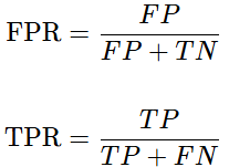
TPR measures how many of the actual positives the model manages to catch, whereas FPR measures how many of the actual negatives the model incorrectly flags as positive.
The resulting metric (AUC) lies in the range of (0,1). If the AUC is 1, then it’s a perfect model; an AUC of 0.5 indicates a random guess, whereas a value less than 0.5 means the model’s predictions are worse than random guessing. Look at the sample ROC curve shown below.
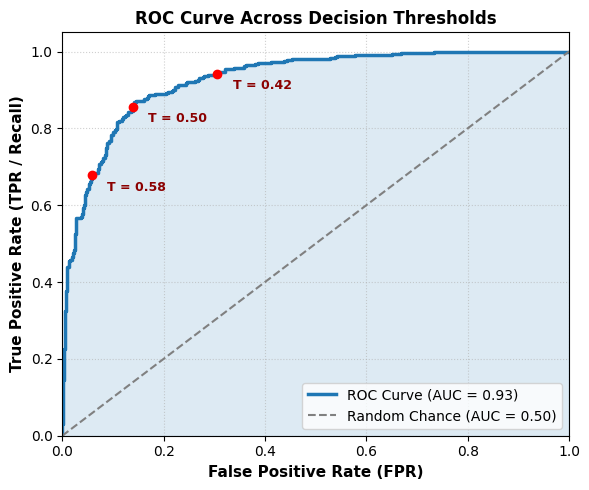
An ROC curve with an {AUC} of 0.93. The red points illustrate how shifting the operational decision threshold (T) directly navigates the trade-off between catching positive cases (TPR) and triggering false alarms (FPR).
Here, in the graph above, the continuous blue curve is built by evaluating all 1,000 unique probability thresholds from the test dataset. Labeling every single cutoff would make the chart completely unreadable. Instead, the diagram highlights just three representative thresholds with red dots to provide concrete examples of the trade-off without cluttering the visual.
When to Use ROC-AUC?
ROC-AUC is useful when:
- You want to evaluate ranking performance across thresholds.
- The classification threshold hasn’t been finalized.
- The model’s overall discrimination ability is needed.
It is important to note that ROC-AUC isn’t always the best choice for highly imbalanced datasets. If positive cases are rare, the false positive rate can remain small even when the model generates a large number of false positives. To overcome this problem, we can use the metric called PR-AUC.
6. PR-AUC
PR-AUC stands for precision-recall area under the curve. While ROC-AUC plots true positive rate versus false positive rate, PR-AUC plots precision versus recall. This is useful when the positive classes are rare.
Imagine a record of 999,000 legitimate and 1,000 fraudulent transactions. But your model raises 5000 false alarms. Here, relying on the ROC curve would give a false positive rate of approximately 0.5%. But because the number of legitimate transactions is massive, 0.5% looks almost negligible, and ROC would give a perfect score. PR-AUC solves this problem by strictly plotting precision against recall across varying classification thresholds.
In simple terms, ROC compares false alarms against the huge sea of 999,000 normal transactions, whereas PR-AUC ignores the normal transactions entirely and asks:
- Recall: How many of the 1,000 real frauds did you catch?
- Precision: Out of the alerts you raised, how many were real versus false alarms (precision)?
When to Use PR-AUC?
PR-AUC is useful when:
- The positive class is rare.
- You’re interested in detecting the positive class.
- False positives matter.
For imbalanced classification problems, it is recommended to use both ROC-AUC and PR-AUC rather than relying on any one. Evaluating both metrics ensures you understand global class separability while preventing high True Negative counts from masking poor precision on rare positive events.
7. Log Loss
Log loss assesses how well the model’s predicted probabilities align with the true labels. This is different from metrics that evaluate whether the model’s predictions are correct.
Consider two models, A and B, for the positive class. Model A shows a 55% probability, whereas B shows a 1% probability. Here, model B was not only wrong but also confident, even with the wrong prediction, and log Loss is designed to capture exactly this scenario. Its mathematical formula for binary classification is:

- N is the number of observations.
- yᵢ is the actual class, either 0 or 1.
- pᵢ is the predicted probability of the positive class.
Log Loss rewards correct predictions and penalises confident incorrect predictions.
- Correct + high confidence → small loss
- Correct + low confidence → larger loss
- Wrong + high confidence → very large loss
A perfectly designed classifier can approach a log loss of near zero.
When to Use Log Loss?
Log Loss is useful when the quality of the predicted probabilities matters, such as:
- Medical risk prediction
- Credit risk scoring
- Insurance risk models
- Recommendation systems
Code Snippet
from sklearn.metrics import precision_score, recall_score, f1_score, roc_auc_score, average_precision_score, log_loss

# Precision, Recall, F1 (Hard labels)
precision = precision_score(y_true, y_pred)
recall = recall_score(y_true, y_pred)
f1 = f1_score(y_true, y_pred)

# ROC-AUC, PR-AUC, Log Loss (Probabilities)
roc_auc = roc_auc_score(y_true, y_pred_proba)
pr_auc = average_precision_score(y_true, y_pred_proba)
loss = log_loss(y_true, y_pred_proba)
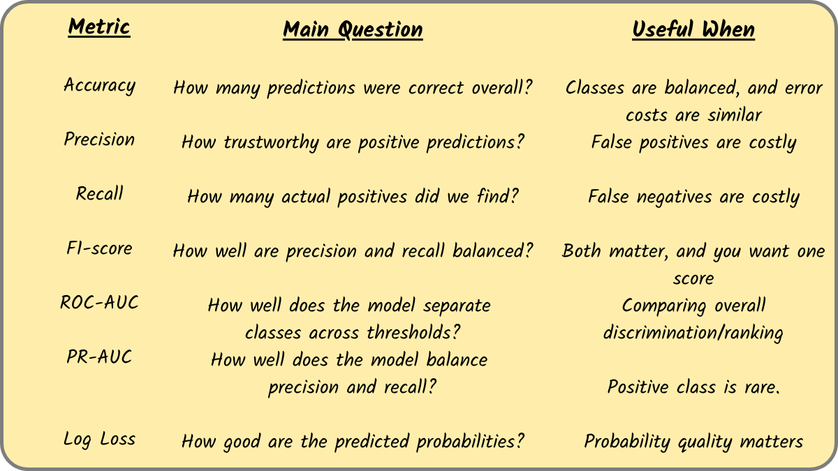
Final Thoughts: When to Choose What?
Opinions expressed by DZone contributors are their own.