Lane Detection With OpenCV (Part 2)
In this article, featuring part 2 of 2, we will see how to detect straight lanes in a road using OpenCV and discuss how to eventually extend it for turns.
Join the DZone community and get the full member experience.
Join For FreeIn the first part, we saw how to select the color of the lanes using thresholding, and how to use perspective correction to get a bird’s eye view or the road. We will now see how to locate the lanes.
The following content is mostly an extract from the book Hands-On Vision and Behavior for Self-Driving Cars, that I wrote for Packt Publishing, with the help of Krishtof Korda.
Edge Detection
The code requires Python 3.7, Matplotlib, OpenCV and NumPy.
The next step is detecting the edges, and we will use the green channel for that, as during our experiments, it gave good results. Please be aware that you need to experiment with the images and videos taken from the country where you plan to run the software, and with many different light conditions. Most likely, based on the color of the lines and the colors in the image, you might want to choose a different channel, possibly from another color space; you can convert the image into different color spaces using cvtColor(), for example:
img_hls = cv2.cvtColor(img_bgr, cv2.COLOR_BGR2HLS).astype(np.float)
We will stick to green.
OpenCV has several ways to compute edge detection, and we are going to use Scharr, as it performs quite well. Scharr computes a derivative, so it detects the difference in colors in the image. We are interested in the X axis, and we want the result to be a 64-bit float, so our call would be like this:
xxxxxxxxxx
edge_x = cv2.Scharr(channel, cv2.CV_64F, 1, 0)
As Scharr computes a derivative, the values can be both positive and negative. We are not interested in the sign, but only in the fact that there is an edge. So, we will take the absolute value:
xxxxxxxxxx
edge_x = np.absolute(edge_x)
Another issue is that the values are not bounded on the 0–255 value range that we expect on a single channel image, and the values are floating points, while we need an 8-bit integer. We can fix both the issues with the following line:
xxxxxxxxxx
edge_x = np.uint8(255 * edge_x / np.max(edge_x))
This is the result:
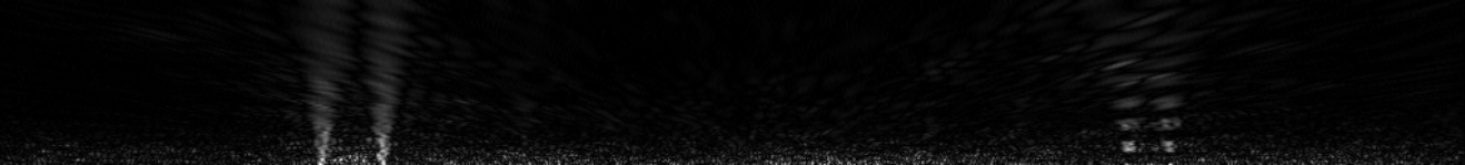
At this point, we can apply thresholding to convert the image into black and white, to better isolate the pixels of the lanes. We need to choose the intensity of the pixels to select, and in this case, we can go for 20–120; we will select only pixels that have at least an intensity value of 20, and not more than 120:
xxxxxxxxxx
binary = np.zeros_like(img_edge)
binary[img_edge >= 20] = 255
The zeros_like() method creates an array full of zeros, with the same shape of the image, and the second line sets all the pixels with an intensity between 20 and 120 to 255. This is the result:
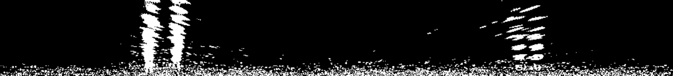
The lanes are now very visible, but there is some noise. We can reduce that by increasing the threshold:
xxxxxxxxxx
binary[img_edge >= 50] = 255
This is how the output appears:
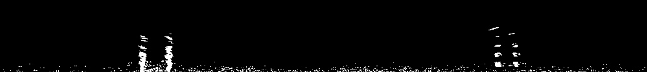
Now, there is less noise, but we lost the lines on the top.
We will now describe a technique that can help us to retain the full line without having an excessive amount of noise.
Interpolated Threshold
In practice, we don’t have to choose between selecting the whole line with a lot of noise and reducing the noise while detecting only part of the line. We could apply a higher threshold to the bottom (where we have more resolution, a sharper image, and more noise) and a lower threshold on the top (there, we get less contrast, a weaker detection, and less noise, as the pixels are stretched by the perspective correction, naturally blurring them). We can just interpolate between the thresholds:
xxxxxxxxxx
threshold_up = 15
threshold_down = 60
threshold_delta = threshold_down-threshold_up
for y in range(height):
binary_line = binary[y,:]
edge_line = channel_edge[y,:]
threshold_line = threshold_up + threshold_delta * y/height
binary_line[edge_line >= threshold_line] = 255
Let’s see the result:
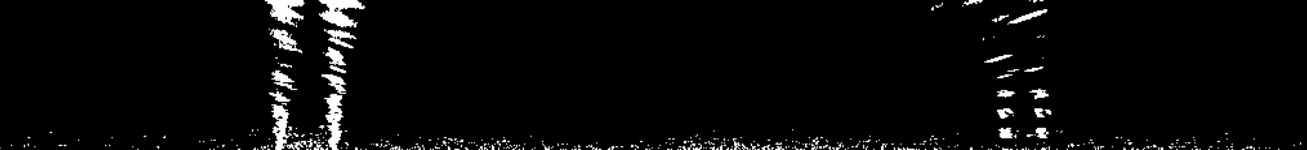
Now, we can have less noise at the bottom and detect weaker signals at the top. However, while a human can visually identify the lanes, for the computer, they are still just pixels in an image, so there is still work to do. But we simplified the image very much, and we are making good progress.
Combined Threshold
As we mentioned earlier, we also wanted to use the threshold on another channel, without edge detection. We chose the L channel of HLS.
This is the result of thresholding above 140:
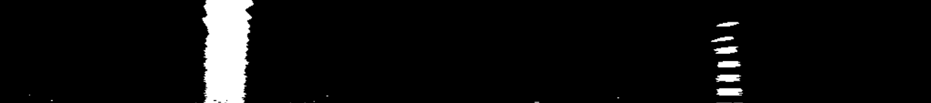
Not bad. Now, we can combine it with the edge:
The result is noisier, but also more robust.
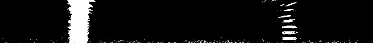
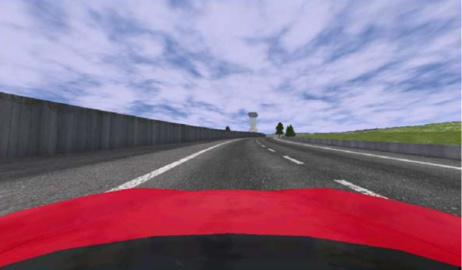
Before moving forward, let’s introduce a picture with a turn:
This is the threshold:
It still looks good, but we can see that, because of the turn, we no longer have a vertical line. In fact, at the top of the image, the lines are basically horizontal
Finding the Lanes Using Histograms
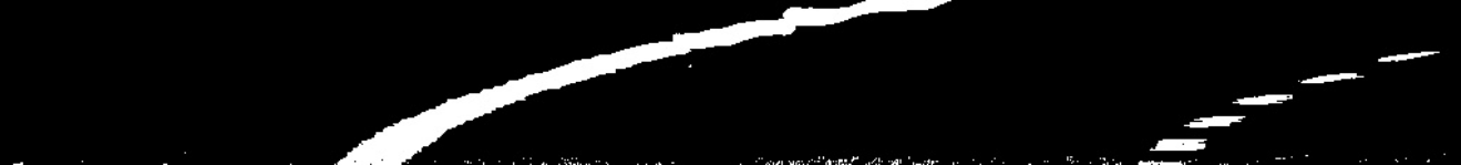
How could we understand, more or less, where the lanes are? Visually, for a human, the answer is simple: the lane is a long line. But what about a computer?
If we talk about vertical lines, one way could be to count the pixels that are white, on a certain column. But if we check the image with a turn, that might not work. However, if we reduce our attention to the bottom part of the image, the lines are a bit more vertical:

We can now count the pixels by column:
xxxxxxxxxx
partial_img = img[img.shape[0] // 2:, :] # Select the bottom part
hist = np.sum(partial_img, axis=0) # axis 0: columns direction
To save the histogram as a graph, in a file, we can use Matplotlib:
xxxxxxxxxx
import matplotlib.pyplot as plt
plt.plot(hist)
plt.savefig(filename)
plt.clf()
We obtain the following result:
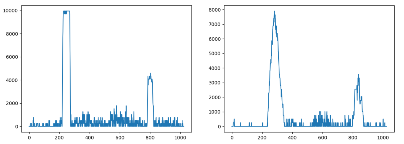
The X coordinates on the histogram represent the pixels; as our image has a resolution of 1024x600, the histogram shows 1,024 data points, with the peaks centered around the pixels where the lanes are.
As we can see, in the case of a straight lane, the histogram identifies the two lines quite clearly; with a turn, the histogram is less clear (because the line makes a turn and, therefore, the white pixels are spread a bit around), but it’s still usable. We can also see that in the case of a dotted line, the peek in the histogram is less pronounced, but it is still there.
This looks promising!
Now, we need a way to detect the two peaks. We can use argmax() from NumPy, which returns the index of the maximum element of an array, which is one of our peaks.
However, we need two. For this, we can split the array into two halves, and select one peak on each one:
xxxxxxxxxx
size = len(histogram)
max_index_left = np.argmax(histogram[0:size//2])
max_index_right = np.argmax(histogram[size//2:]) + size//2
Now we have the indexes, which represent the X coordinate of the peaks. The value itself (for example, histogram[index]) can be considered the confidence of having identified the lane, as more pixels mean more confidence.
Last Words
Now you know the initial position of the lane. The remaining chapter of the book explains how to enhance this method to identify turns (moving the window used to compute the histograms), how to draw a line on the identified lanes, and how to leverage information from the previous frames to make the detection more robust.
If you liked these two articles and if you are curious about some of the technologies used by self-driving cars, please consider the Hands-On Vision and Behavior for Self-Driving Cars book. It talks also about Neural Networks, Object Detection, Semantic Segmentation, sensors, lidars, maps, control and more.
Published at DZone with permission of Luca Venturi. See the original article here.
Opinions expressed by DZone contributors are their own.
Comments