Linear Regression Using Numpy
By
 ·
·
Interview
·
·
Interview
Likes
(0)
Likes
There are no likes...yet! 👀
Be the first to like this post!
It looks like you're not logged in.
Sign in to see who liked this post!
Comment
Save
14.0K Views
Join the DZone community and get the full member experience.
Join For FreeA few posts ago, we saw how to use the function
numpy.linalg.lstsq(...) to solve an over-determined system. This time,
we'll use it to estimate the parameters of a regression line.
A linear regression line is of the form w1x+w2=y and it is the line that minimizes the sum of the squares of the distance from each data point to the line. So, given n pairs of data (xi, yi), the parameters that we are looking for are w1 and w2 which minimize the error

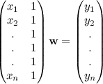
and we can compute the parameter vector w = (w1 , w2)T as the least-squares solution of the following over-determined system

Let's use numpy to compute the regression line:

You can find more about data fitting using numpy in the following posts:
A linear regression line is of the form w1x+w2=y and it is the line that minimizes the sum of the squares of the distance from each data point to the line. So, given n pairs of data (xi, yi), the parameters that we are looking for are w1 and w2 which minimize the error
and we can compute the parameter vector w = (w1 , w2)T as the least-squares solution of the following over-determined system
Let's use numpy to compute the regression line:
from numpy import arange,array,ones,random,linalg
from pylab import plot,show

xi = arange(0,9)
A = array([ xi, ones(9)])
# linearly generated sequence
y = [19, 20, 20.5, 21.5, 22, 23, 23, 25.5, 24]
w = linalg.lstsq(A.T,y)[0] # obtaining the parameters

# plotting the line
line = w[0]*xi+w[1] # regression line
plot(xi,line,'r-',xi,y,'o')
show()
We can see the result in the plot below.

You can find more about data fitting using numpy in the following posts:
Linear regression
NumPy
Published at DZone with permission of Giuseppe Vettigli. See the original article here.
Opinions expressed by DZone contributors are their own.
Comments