Predicting Traffic Volume With Artificial Intelligence and Machine Learning

Effective traffic forecasting is important for urban planning, especially in reducing congestion, improving traffic flow, and maintaining public safety. This study examines the performance of machine learning models of linear regression, decision trees, and random forest to predict traffic flow along the westbound I-94 highway, using datasets collected between 2012 and 2018.

Exploratory data analysis revealed traffic volume patterns related to weather, holidays, and time of day. The models were evaluated based on R2 and mean squared error (MSE) metrics, with random forest outperforming others, obtaining an R2 of 0.849 and lower MSE than linear regression and decision tree models. 

This study highlights the potential of random forest models in traffic forecasting and provides insights for future research aimed at improving urban traffic management systems.

Introduction

Effective traffic forecasting is crucial for modern city management, serving as a factor in efforts to reduce congestion, improve traffic flow, and enhance public safety. With urban areas growing at unprecedented rates, traditional methods of traffic prediction are often insufficient to address the complexities of modern traffic dynamics. Recent advances in machine learning have opened new avenues for enhancing the accuracy of traffic forecasts. For instance, Da Zhang and Mansur R. Kabuka (2018) demonstrated the power of a GRU-based deep learning approach that integrates weather conditions to predict urban traffic flow, achieving notable improvements in predictive accuracy and error reduction compared to previous methods. Similarly, Alex Lewis, Rina Azoulay, and Esther David (2020) showcased the efficacy of ensemble methods and K-Nearest Neighbors (KNN) in forecasting traffic speed, offering superior accuracy and consistency that can significantly benefit traffic management.

Building on these advancements, this paper investigates the performance of simpler models such as linear regression, decision trees, and random forest models in predicting traffic volume on the westbound I-94 highway. By evaluating and comparing these machine learning models, the paper aims to identify the most reliable yet simple approach for practical application in traffic management systems.

Dataset

The dataset contains hourly data on traffic on westbound I-94, the major interstate highway connecting Minneapolis and St. Louis. Paul, Minnesota. This data was collected by the Minnesota Department of Transportation (MNDOT) from 2012 to 2018 at a station that is between the two cities. This dataset has a number of columns capturing traffic volume and weather patterns that span multiple years to provide a comprehensive view of long-term traffic patterns.

Our dataset contains 48,204 rows, each representing a separate hourly observation, enabling detailed analysis of traffic patterns and their relationship over a seven-year period of time. Key characteristics in the data set include:

• holiday, a categorical variable indicating whether the date is a US national or regional holiday
• temp, a numerical variable representing temperature in Kelvin 
• rain_1h and snow_1h, statistical variables indicating the amount of rain and snow in millimeters that occurred in the last hour, respectively
• clouds_all, a statistical variable indicating the percentage of cloud cover
• weather_main and weather_description, categorical variables providing short and long descriptions of the current weather
• date_time, a DateTime variable specifying the hour of data collection at the local CST time
• traffic_volume, a statistical variable representing the reported hourly traffic volume for westbound I-94

We split the date_time column into separate columns for year, month, day, and hour. This method ensures that each component of the date and time is accurately extracted and stored in a new column.

Exploratory Data Analysis (EDA)

In this section, exploratory data analysis (EDA) is conducted to understand the relationships within the data, identify patterns and trends, and extract valuable insights. Figure 1 displays the distribution of traffic volume, with the x-axis representing traffic volume ranging from 0 to 7,000 and the y-axis showing the count of occurrences. There is a notable peak in the low traffic volume range (0-1,000), followed by several smaller peaks around 3,000, 4,000, and 5,000. The distribution is multimodal, indicating multiple common traffic volume levels.

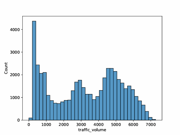
Figure 1: Traffic volume distribution

Figure 2 illustrates the difference in traffic volume on holidays compared to non-holiday days. Non-holiday days show significantly higher and more variable traffic volumes compared to holidays. Each holiday, such as Christmas Day, New Year's Day, and Thanksgiving Day, has a distinct box plot showing the median, IQR, and range of traffic volumes. Figure 2 highlights a substantial drop in traffic volume on holidays, suggesting that holidays lead to a noticeable reduction in traffic.

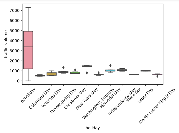
Figure 2: Traffic volume compared to holidays and not holidays

Figure 3 compares traffic volume distributions across various weather conditions such as clouds, clear, rain, and more. Each box represents the IQR, median, and range of traffic volumes for a specific weather type. Figure 3 shows that traffic volume is generally higher and more consistent under clear and cloudy conditions, while it is lower and more variable during snow, squall, and smoke conditions. This indicates that certain weather conditions can lead to more significant variations in traffic volume.

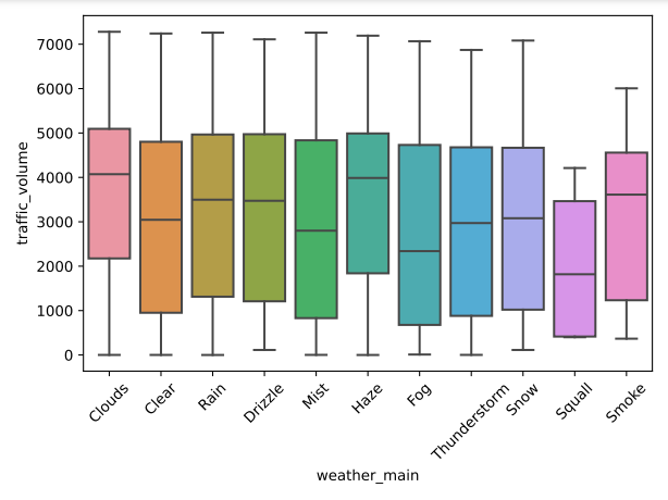
Figure 3: Traffic volume compared to weather

Figure 4 displays the distribution of traffic volume for different snowfall amounts in the last hour, ranging from 0.0 to 0.51 mm. Figure 4 shows that traffic volume generally decreases with increasing snowfall, particularly at moderate levels like 0.13 mm. The variability in traffic volume increases with higher snowfall amounts, indicating that snow may or may not significantly impact traffic patterns.

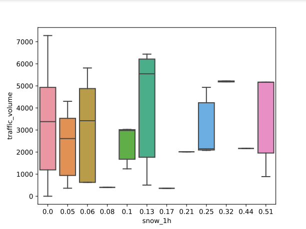
Figure 4: Traffic volume compared to snow levels

Figure 5 shows traffic volume from 2012 to 2019, color-coded by weather conditions such as clouds, clear, rain, and more. Each point represents traffic volume at a specific time under a particular weather condition. The plot illustrates that traffic volume remains consistently high over the years, with no dramatic drops during any specific weather condition. The dense distribution of points causes the challenge to identify the weather conditions that may impact the overall traffic volume.

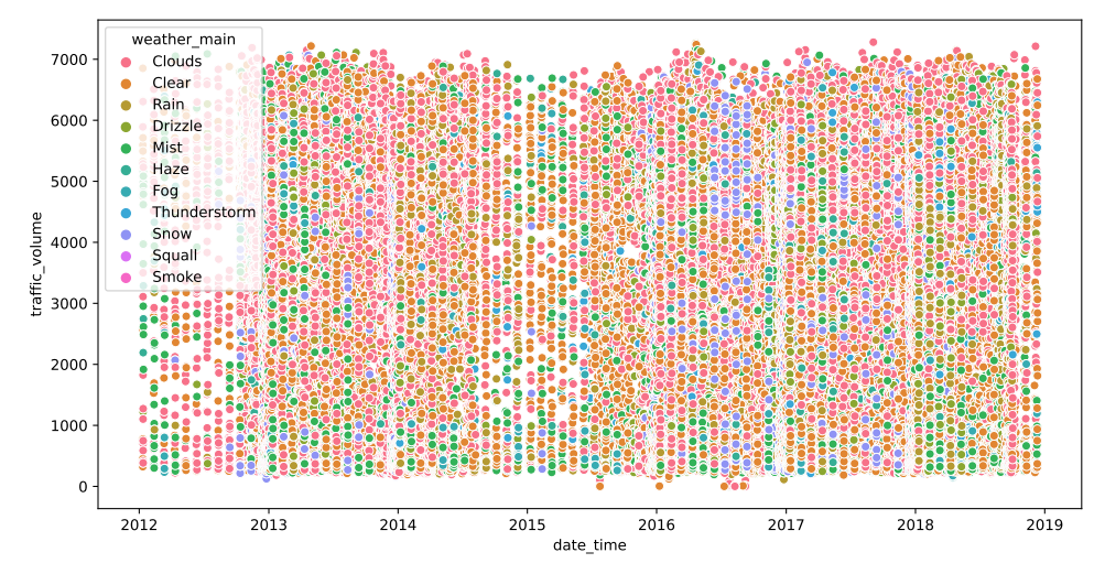
Figure 5: Weather as a function of time

Figure 6 depicts traffic volume across different days of the week, revealing that Friday experiences the highest median traffic volume, suggesting a busier end to the work week. In comparison, Saturday and Sunday have the lowest median traffic volumes, indicating lighter weekend traffic. Overall, traffic volumes are more consistent and higher during weekdays, with less fluctuation and lower volumes on weekends.

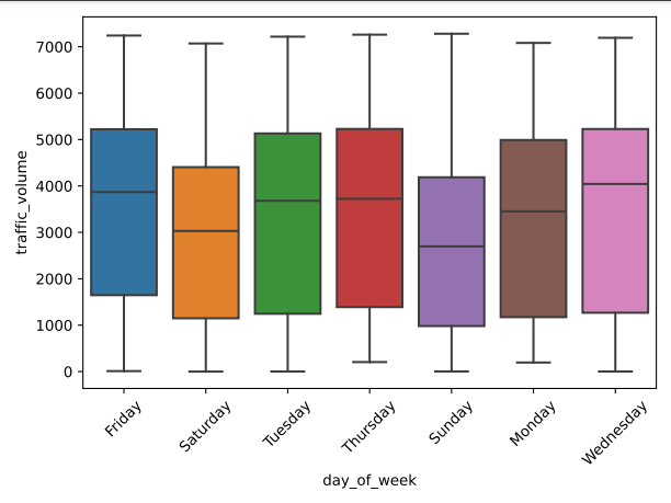
Figure 6: Traffic volume compared to day of week

Figure 7 shows traffic volume by hour of the day, with notable peaks during the morning rush hours (6-9 AM) and evening rush hours (3-6 PM), indicating heavy commuting periods. The traffic volume is lowest from midnight to early morning (12-4 AM), with a gradual increase starting around 5 AM and a gradual decrease after 6 PM. This pattern highlights typical daily commuting behavior, with significant variations throughout the day.

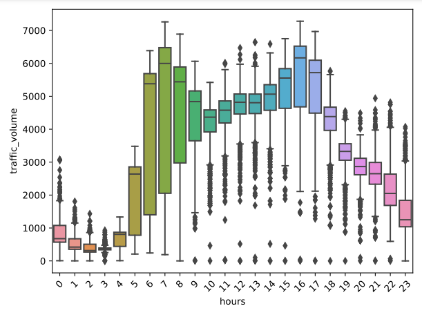
Figure 7: Traffic volume compared to time of day

Models and Methods

Our target is traffic volume, and input features are holiday, temp, rain_1h, snow_1h, clouds_all, weather_main, and day_of_week. In this study, the categorical columns weather_main, holiday, and day_of_week category columns are converted to numeric values using hot encoding. For example, holiday is converted to true and false values. One-hot encoding is a method of converting categorical variables into a format that can be fed to machine learning algorithms. It converts each class value into a new class column and assigns a new value indicating its presence or absence in that class data. 

The data was split into two parts, one for training and the other for testing. Specifically, 20% of the data was allocated to the test set, while the remaining 80% was used to train the model. This approach allows the model to be built and refined using the training set, followed by an evaluation of its performance on the test set to ensure it generalizes well to new, unseen data. To maintain consistency across different code runs, the random_state was fixed, ensuring that the data is evenly distributed each time. This reproducibility is crucial for reliable model evaluation and comparison.

In this study, linear regression, decision trees, and random forest models were implemented. Linear regression is a statistical technique that models the relationship between a dependent variable and one or more independent variables by establishing a linear relationship to the data. The goal is to find the best-fitting line that minimizes the sum of the squared differences between the observed and predicted values. The equation of the line is y=β0+β1x1+…+βnxn, where β coefficients are determined using the data. Although simple and widely used, linear regression assumes linear relationships and can be affected by outliers.

A decision tree is a machine learning algorithm for classification and regression tasks. It works by repeatedly dividing the data into smaller units based on the values of the input features, forming a tree-like structure in which each node represents a test on the feature, each branch represents a test result, and each leaf node represents a class label or a continuous value. The goal is to build models that predict target variables by learning simple decision rules from the data components. Decision trees are easy to define and visualize but can be prone to over-interaction, especially with complex data sets.

The random forest model is a group learning method used for classification and regression applications that generates multiple decision trees during training and combines the results for more accurate static forecasts. Each tree in the forest is trained on discrete data with small random features, which helps reduce overfitting and improves generalization Random forests are very efficient and are difficult, but potentially more computationally intensive and less interpretable compared to single decision trees.

Evaluation methods are important for evaluating the performance of models, and two commonly used metrics are R-squared (R2) and mean-squared error (MSE). R2 measures the proportion of the variance in the dependent variable that is predictable from the independent variables, the results being between 0 and 1. The higher the value, the better the results. MSE, on the other hand, quantifies the average squared difference between the predicted and actual values, with lower values indicating more accurate predictions. Although R2 provides a measure of fit, MSE provides a stronger understanding of forecast error size and helps to measure how well the model performs in terms of accuracy and precision.

Hyperparameter tuning is the process of optimizing the performance of machine learning models by systematically evaluating a range of default values for specific parameters. We hyperparameters tuned the baseline random forest model. In this case, the parameters being mined are n_estimators, which take into account the number of trees in the cluster, with possible values of 500 and 1000; max_features, specifying the number of features to consider by finding the best partition, from 1 to 4; and min_samples_split, which specifies the minimum number of samples needed to split the nodes, ranging from 20 to 150 in increments of 10. Using these parameters, the goal is to find the combination that gives the best model performance.

Results and Discussion

Table 1 provides a comparison of three baseline models: linear regression, decision tree, and random forest, based on their performance measures — R² and MSE (mean squared error) for both training and testing datasets. Linear regression reveals low R² values (0.164 for training and 0.167 for testing) and high MSE values (more than 3 million), indicating poor quality and poor prediction performance. The decision tree model is almost well suited for training data (R² of 0.999) but significantly reduced test performance (R2 of 0.758) means, with increased MSE, indicating overfitting. The random forest model is well balanced, with high R² values (0.978 for training and 0.849 for testing) and low MSE values compared to the decision tree, indicating good generalization and prediction accuracy, but exhibiting slight overfitting as well.

These results indicate that while the decision tree can model the training data very well, it struggles with new data due to overfitting. The random forest, however, generalizes better to unseen data, providing more consistent and accurate predictions. This means that for practical applications, the hyperparameter-tuned random forest model is likely to be more effective and dependable than the other models tested. Making it a more reliable model for predicting traffic volume compared to both the decision tree and linear regression models. 

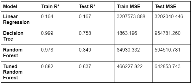
Table 1: Evaluation metrics of baseline models and hyperparameter-tuned model

Figure 8 shows the performance of the basic linear regression model in forecasting traffic volume. Each point in the plot represents a forecast, with the predicted traffic volume on the y-axis and the actual traffic volume on the x-axis. In contrast to more sophisticated models, this plot's points show notable differences between the true and predicted values by forming a horizontal band instead of grouping along the diagonal line. This pattern highlights the limitations of the linear regression model in capturing the complexity of the underlying data patterns and its tendency to produce predictions that do not align well with the true traffic volumes. It also suggests that the model's predictions are less accurate and show significant variability. 

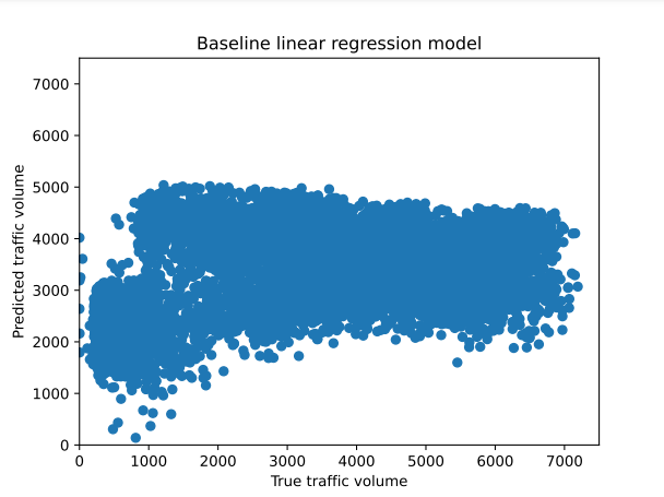
Figure 8. Actual vs. predicted traffic volume, using baseline linear regression model

Figure 9 shows the performance of the basic decision tree model for predicting traffic density. Similar to the figure in Figure 8, each point represents a prediction, with the predicted number of vehicles on the y-axis and the actual number of vehicles on the x-axis In contrast to the random forest, the points are widely scattered and not the diagonal lines of many clusters. This indicates that the decision tree model's predictions are less accurate and more variable, highlighting its tendency to overfit the training data, resulting in poorer generalization to new, unseen data.

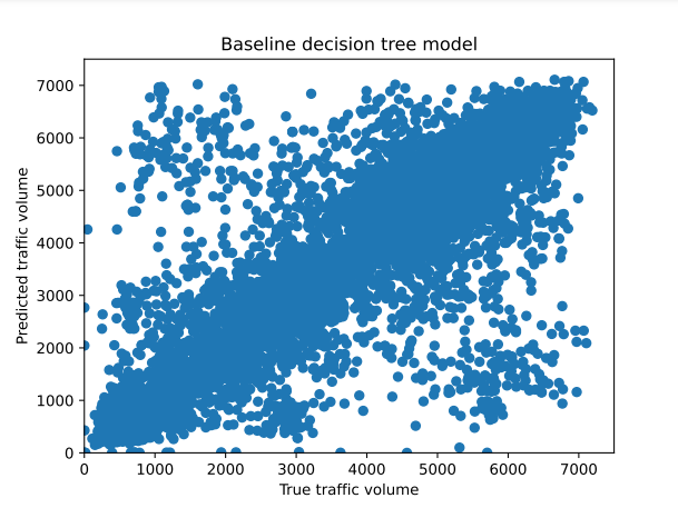
Figure 9: Actual vs. predicted traffic volume, using baseline decision tree model

Figure 10 shows the performance of the baseline random forest model to predict the number of vehicles. Like Figure 8, each case represents a forecast, where the predicted traffic volume is plotted against the actual traffic volume. The plot shows that the points along the diagonal line overlap strongly, indicating that the predictions of the random forest model tend to be closer to the actual values. This suggests that the random forest model is effective in capturing the patterns in the data, leading to accurate traffic volume predictions.

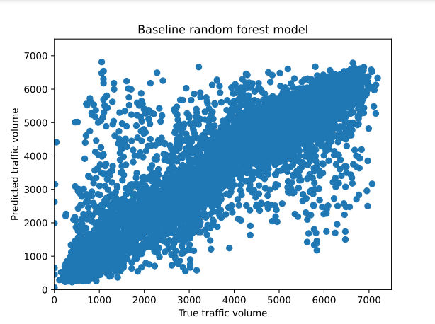
Figure 10: Actual vs. predicted traffic volume, using baseline random forest model

After hyperparameter tuning of the baseline random forest model, the best model was determined by the parameters: max_features set to 4, min_samples_split set to 20, and n_estimators set to 1000. This setting provided a balance between model complexity and generalization was successful, resulting in 0.8818 train R-squared, and train mean squared error (MSE) of 466,227.82. During the testing process, the model obtained an R-square of 0.8374 and an MSE of 642,853.74. The difference between training and testing metrics indicates that overfitting was effectively reduced, as the model performed well on unseen data, reduced error rates, and maintained strong predictive power

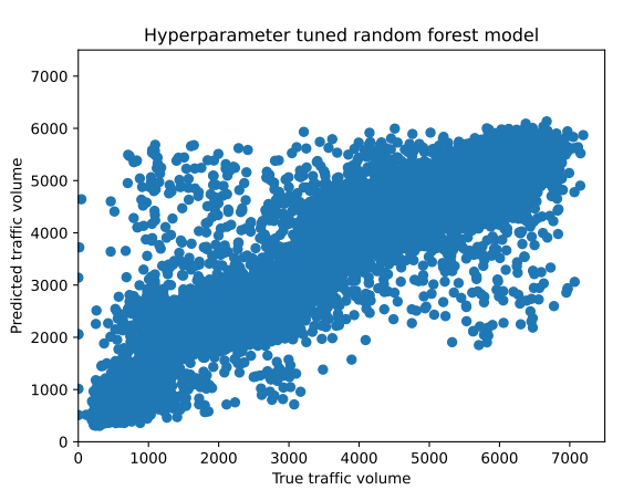
Figure 11: Actual vs. predicted traffic volume, using hyperparameter-tuned random forest model

Conclusions

In conclusion, this study assessed how well three machine learning models performed in terms of forecasting traffic flow on the westbound I-94 highway: random forest, decision tree, and linear regression. The results of the investigation showed that the decision tree model showed considerable overfitting, performing well on the training data but badly on the test data, while linear regression found it difficult to capture the complexity of the traffic data, resulting in poor prediction performance. The random forest model, on the other hand, showed better predictive accuracy and generalization capacity, successfully striking a better balance between fitting and efficacy across training and testing datasets. These findings highlight the importance of applying random forest-like methods to the modeling of complex, real-world phenomena such as traffic density, where it is important they capture complex patterns and ensure good performance on new data. 

Precise prediction of traffic volume is essential for efficient traffic control and urban planning, as it aids in easing traffic, streamlining traffic, and cutting down on journey durations. Authorities can make better decisions concerning emergency response plans, infrastructure development, and traffic control measures by increasing the accuracy of traffic predictions. In order to improve forecast accuracy and offer more thorough insights into traffic dynamics, future research might investigate further model optimization and the addition of new factors, which would ultimately lead to the development of more sustainable and effective transportation systems.