Exploring Decision Trees: A Beginner's Guide
Explore fundamental concepts of decision trees, including entropy, information gain, and Gini impurity, which form the basis of their decision-making process.
Join the DZone community and get the full member experience.
Join For FreeIf you're eager to learn or understand decision trees, I invite you to explore this article. Alternatively, if decision trees aren't your current focus, you may opt to scroll through social media.
About Decision Trees
![Simple decision tree]()
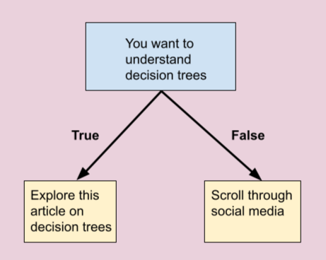
Figure 1: Simple Decision tree
The image above shows an example of a simple decision tree. Decision trees are tree-shaped diagrams used for making decisions based on a series of logical conditions. In a decision tree, each node represents a decision statement, and the tree proceeds to make a decision based on whether the given statement is true or false.
There are two main types of decision trees: Classification trees and Regression trees. A Classification tree categorizes problems by classifying the output of the decision statement into categories using if-else logical conditions. Conversely, a Regression tree classifies the output into numeric values.
In Figure 2, the topmost node of a decision tree is called the Root node, while the nodes following the root node are referred to as Internal nodes or branches. These branches are characterized by arrows pointing towards and away from them. At the bottom of the tree are the Leaf nodes, which carry the final classification or decision of the tree. Leaf nodes are identifiable by arrows pointing to them, but not away from them.
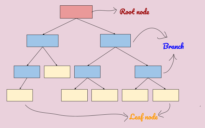
Figure 2: Nodes of a Decision tree
Primary Objective of Decision Trees
The primary objective of a decision tree is to partition the given data into subsets in a manner that maximizes the purity of the outcomes.
Advantages of Decision Trees
- Simplicity: Decision trees are straightforward to understand, interpret, and visualize.
- Minimal data preparation: They require minimal effort for data preparation compared to other algorithms.
- Handling of data types: Decision trees can handle both numeric and categorical data efficiently.
- Robustness to non-linear parameters: Non-linear parameters have minimal impact on the performance of decision trees.
Disadvantages of Decision Trees
- Overfitting: Decision trees may overfit the training data, capturing noise and leading to poor generalization on unseen data.
- High variance: The model may become unstable with small variations in the training data, resulting in high variance.
- Low bias, high complexity: Highly complex decision trees have low bias, making them prone to difficulties in generalizing new data.
Important Terms in Decision Trees
Below are important terms that are also used for measuring impurity in decision trees:
1. Entropy
Entropy is a measure of randomness or unpredictability in a dataset. It quantifies the impurity of the dataset. A dataset with high entropy contains a mix of different classes or categories, making predictions more uncertain.
- Example: Consider a dataset containing data from various animals as in Figure 3. If the dataset includes a diverse range of animals with no clear patterns or distinctions, it has high entropy.
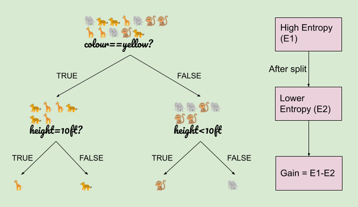
Figure 3: Animal datasets
2. Information Gain
Information gain is the measure of the decrease in entropy after splitting the dataset based on a particular attribute or condition. It quantifies the effectiveness of a split in reducing uncertainty.
- Example: When we split the data into subgroups based on specific conditions (e.g., features of the animals) like in Figure 3, we calculate information gain by subtracting the entropy of each subgroup from the entropy before the split. Higher information gain indicates a more effective split that results in greater homogeneity within subgroups.
3. Gini Impurity
Gini impurity is another measure of impurity or randomness in a dataset. It calculates the probability of misclassifying a randomly chosen element if it were randomly labeled according to the distribution of labels in the dataset. In decision trees, Gini impurity is often used as an alternative to entropy for evaluating splits.
- Example: Suppose we have a dataset with multiple classes or categories. The Gini impurity is high when the classes are evenly distributed or when there is no clear separation between classes. A low Gini impurity indicates that the dataset is relatively pure, with most elements belonging to the same class.
Classifications and Variations
Implementation in Python
The following is used to predict the Lung_cancer of the patients.
1. Importing necessary libraries for data analysis and visualization in Python:
import pandas as pd
import numpy as np
import matplotlib.pyplot as plt
import seaborn as sns

# to ensure plots are displayed inline in Notebook
%matplotlib inline

# Set Seaborn style for plots
sns.set_style("whitegrid")

# Set default Matplotlib style
plt.style.use("fivethirtyeight")
2. Uploading the CSV file containing the data and loading:
import pandas as pd
# Load the data from the CSV file
df = pd.read_csv('survey_lung_cancer.csv')df.head()
# Displaying first five rows of the dataframe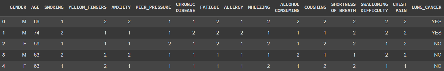
sns.countplot(x='LUNG_CANCER', data=df)
# Count plot using Seaborn
# to visualize the distribution of values in "LUNG_CANCER" column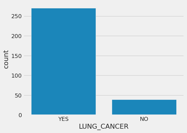
# title AGE

from matplotlib import pyplot as plt
df['AGE'].plot(kind='hist', bins=20, title='AGE')
plt.gca().spines[['top', 'right',]].set_visible(False)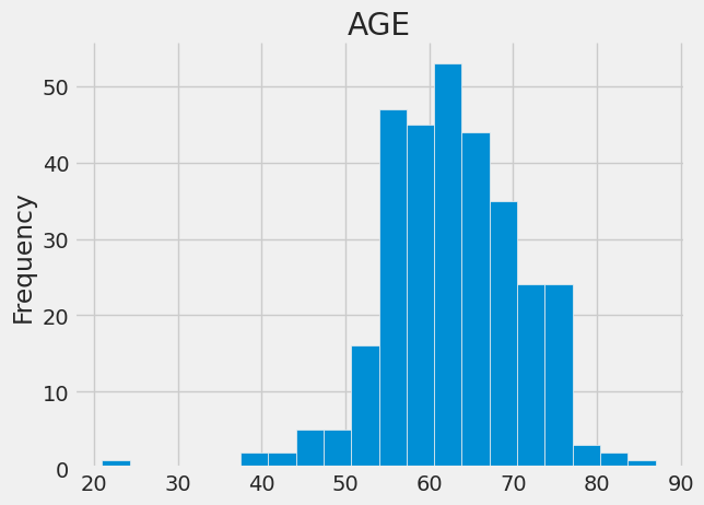
3. Iterating through columns, identifying categorical columns, and appending:
categorical_col = []
for column in df.columns:
    if df[column].dtype == object and len(df[column].unique()) <= 50:
        categorical_col.append(column)

df['LUNG_CANCER'] = df.LUNG_CANCER.astype("category").cat.codes
4. Removing the column "LUNG_CANCER" for further processing:
categorical_col.remove('LUNG_CANCER')5. Encoding categorical variables using LabelEncoder:
from sklearn.preprocessing import LabelEncoder

# creating an instance of the LabelEncoder class
# LabelEncoder will be used to transform categorical values into numerical labels
label = LabelEncoder()
for column in categorical_col:
    df[column] = label.fit_transform(df[column])
6. Dataset splitting for Machine Learning, train_test_split:
from sklearn.model_selection import train_test_split

# X contains the features (all columns except 'LUNG_CANCER')
# y contains the target variable ('LUNG_CANCER') from the DataFrame df
X = df.drop('LUNG_CANCER', axis=1)
y = df.LUNG_CANCER

# performing the Split
X_train, X_test, y_train, y_test = train_test_split(X, y, test_size=0.3, random_state=42)
7. Function for model evaluation and reporting: Overall, the function below serves as a convenient tool for assessing the performance of classification models and generating detailed reports, facilitating model evaluation and interpretation.
# import functions from scikit-learn for model evaluation
from sklearn.metrics import accuracy_score, confusion_matrix, classification_report

# clf: The classifier model to be evaluated
# X_train, y_train: The features and target variable of the training set
# X_test, y_test: The features and target variable of the testing set
def print_score(clf, X_train, y_train, X_test, y_test, train=True):
    if train:
        pred = clf.predict(X_train)
        clf_report = pd.DataFrame(classification_report(y_train, pred, output_dict=True))
        print("Train Result:\n_________________________")
        print(f"Accuracy Score: {accuracy_score(y_train, pred) * 100:.2f}%")
        print("_________________________")
        print(f"CLASSIFICATION REPORT:\n{clf_report}")
        print("_________________________________________________________________________")
        print(f"Confusion Matrix: \n {confusion_matrix(y_train, pred)}\n")

    elif train==False:
        pred = clf.predict(X_test)
        clf_report = pd.DataFrame(classification_report(y_test, pred, output_dict=True))
        print("\nTest Result:\n_________________________")
        print(f"Accuracy Score: {accuracy_score(y_test, pred) * 100:.2f}%")
        print("_________________________")
        print(f"CLASSIFICATION REPORT:\n{clf_report}")
        print("_________________________________________________________________________")
print(f"Confusion Matrix: \n {confusion_matrix(y_test, pred)}\n")- Training and evaluation of decision tree classifier: Overall, this code provides a comprehensive evaluation of the decision tree classifier's performance on both the training and testing sets, including the accuracy score, classification report, and confusion matrix for each set.
During the training process, the decision tree algorithm uses entropy and information gain to recursively split nodes and build a tree that maximizes information gain at each step.
from sklearn.tree import DecisionTreeClassifier

tree_clf = DecisionTreeClassifier(random_state=42)
tree_clf.fit(X_train, y_train)

print_score(tree_clf, X_train, y_train, X_test, y_test, train=True)
print_score(tree_clf, X_train, y_train, X_test, y_test, train=False)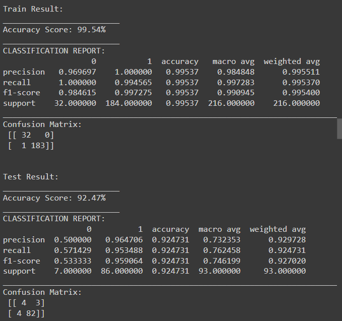
The results above indicate that the decision tree classifier achieved high accuracy and performance on the training set, with some level of overfitting as evident from the difference in performance between the training and testing sets. While the classifier performed well on the testing set, there is room for improvement, particularly in terms of reducing false positives and false negatives. Further tuning of hyperparameters or exploring other algorithms may help improve generalization performance.
8. Visualization of decision tree classifier:
# Importing Dependencies
# Image is used to display images in the IPython environment
# StringIO is used to create a file-like object in memory
# export_graphviz is used to export the decision tree in Graphviz DOT format
# pydot is used to interface with the Graphviz library

from IPython.display import Image
from six import StringIO
from sklearn.tree import export_graphviz
import pydot

features = list(df.columns)
features.remove("LUNG_CANCER")dot_data = StringIO()
export_graphviz(tree_clf, out_file=dot_data, feature_names=features, filled=True)
graph = pydot.graph_from_dot_data(dot_data.getvalue())
Image(graph[0].create_png())
9. Training and evaluation of Random Forest classifier:
from sklearn.ensemble import RandomForestClassifier
# Creating an instance of the Random Forest classifier with n_estimators=100
# which specifies the number of decision trees in the forest
rf_clf = RandomForestClassifier(n_estimators=100)
rf_clf.fit(X_train, y_train)

print_score(rf_clf, X_train, y_train, X_test, y_test, train=True)
print_score(rf_clf, X_train, y_train, X_test, y_test, train=False)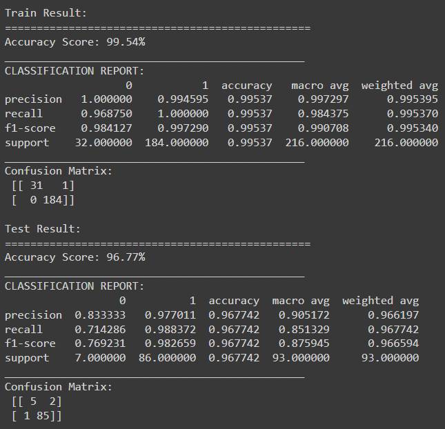
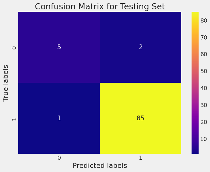
This code below will generate heatmaps for both the training and testing sets' confusion matrices. The heatmaps use different shades to represent the counts in the confusion matrix. The diagonal elements (true positives and true negatives) will have higher values and appear lighter, while off-diagonal elements (false positives and false negatives) will have lower values and appear darker.
import seaborn as sns
import matplotlib.pyplot as plt

# Create heatmap for training set
plt.figure(figsize=(8, 6))
sns.heatmap(cm_train, annot=True, fmt='d', cmap='viridis', annot_kws={"size": 16})
plt.title('Confusion Matrix for Training Set')
plt.xlabel('Predicted labels')
plt.ylabel('True labels')
plt.show()

# Create heatmap for testing set
plt.figure(figsize=(8, 6))
sns.heatmap(cm_test, annot=True, fmt='d', cmap='plasma', annot_kws={"size": 16})
plt.title('Confusion Matrix for Testing Set')
plt.xlabel('Predicted labels')
plt.ylabel('True labels')
plt.show()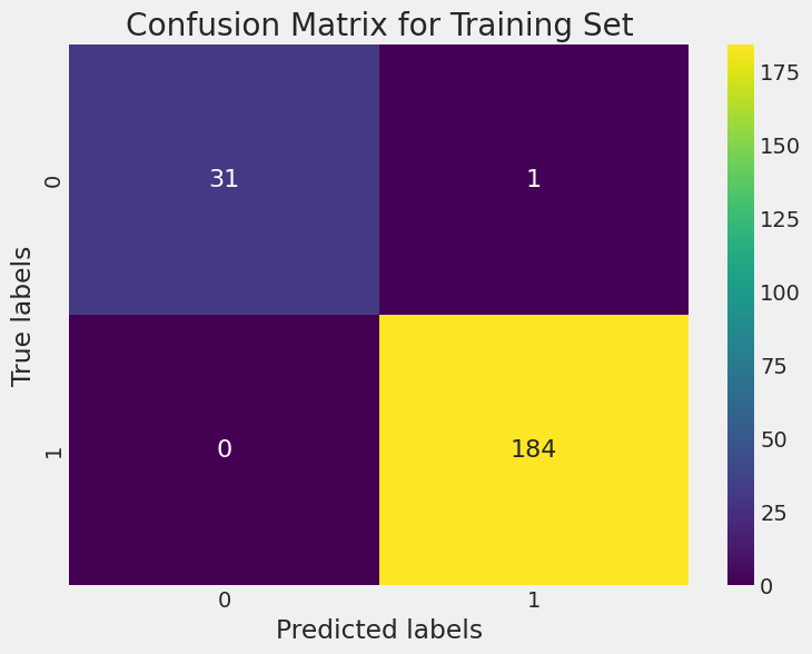
XGBoost for Classification
from xgboost import XGBClassifier
from sklearn.metrics import accuracy_score

# Instantiate XGBClassifier
xgb_clf = XGBClassifier()

# Train the classifier
xgb_clf.fit(X_train, y_train)

# Predict on the testing set
y_pred = xgb_clf.predict(X_test)

# Evaluate accuracy
accuracy = accuracy_score(y_test, y_pred)
print("Accuracy:", accuracy)
The accuracy above indicates that the model's predictions align closely with the actual class labels, demonstrating its effectiveness in distinguishing between the classes.
This code below will generate a bar plot showing the relative importance of the top features in the XGBoost model. The importance is typically calculated based on metrics such as gain, cover, or frequency of feature usage across all trees in the ensemble.
from xgboost import plot_importance
import matplotlib.pyplot as plt

# Plot feature importance
plt.figure(figsize=(10, 6))
plot_importance(xgb_clf, max_num_features=10)
# Specify the maximum number of features to show
plt.show()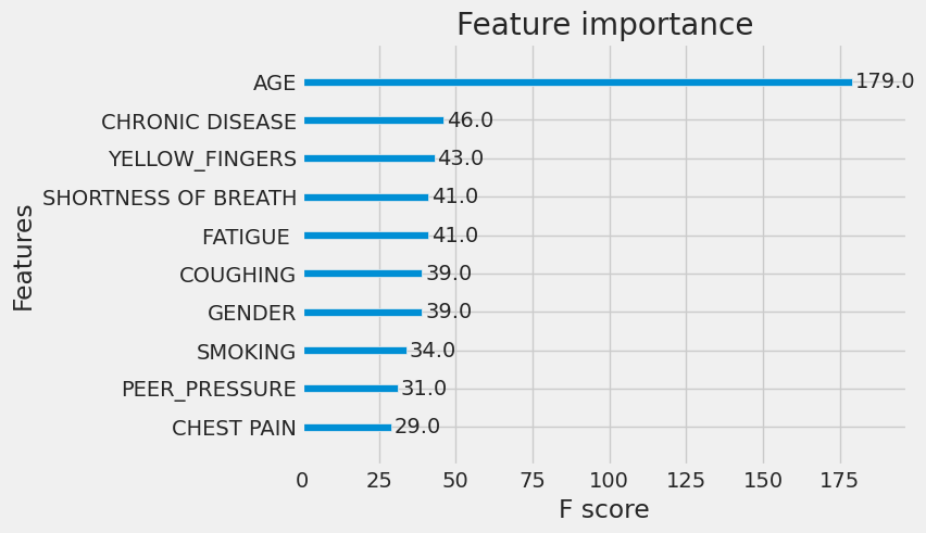
10. Plotting the first tree in the XGBoost model:
from xgboost import plot_tree

# Plot the first tree
plt.figure(figsize=(10, 20))
plot_tree(xgb_clf, num_trees=0, rankdir='TB')
# Specify the tree number to plot
plt.show()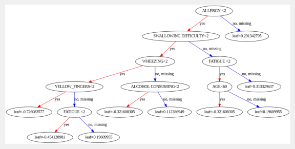
Conclusion
In conclusion, this article gives an idea about how decision trees and their advanced variants like Random Forest and XGBoost offer powerful tools for classification and regression machine learning tasks. Through this journey, we've explored the fundamental concepts of decision trees, including entropy, information gain, and Gini impurity, which form the basis of their decision-making process.
As we continue to delve deeper into the realm of machine learning, the versatility and effectiveness of decision trees and their variants underscore their significance in solving real-world problems across diverse domains. Whether it's classifying medical conditions, predicting customer behavior, or optimizing business processes, decision trees remain a cornerstone in the arsenal of machine learning techniques, driving innovation and progress in the field.
Opinions expressed by DZone contributors are their own.
Comments