Overview of Classical Time Series Analysis: Techniques, Applications, and Models
Explore what makes time series analysis unique and the specialized techniques and models needed to understand and predict future patterns or trends.
Join the DZone community and get the full member experience.
Join For FreeTime series data represents a sequence of data points collected over time. Unlike other data types, time series data has a temporal aspect, where the order and timing of the data points matter. This makes time series analysis unique and requires specialized techniques and models to understand and predict future patterns or trends.
Applications of Time Series Modeling
Time series modeling has a wide range of applications across various fields including:
- Economic and financial forecasting: Predicting future stock prices, volatility, and market trends; Forecasting GDP, inflation, and unemployment rates
- Risk management: Assessing and managing financial risk through Value at Risk (VaR) models
- Weather forecasting: Predicting short-term weather conditions such as temperature and precipitation
- Climate modeling: Analyzing long-term climate patterns and predicting climate change impacts
- Epidemiology: Tracking and predicting the spread of diseases
- Patient monitoring: Analyzing vital signs and predicting health events such as heart attacks
- Demand forecasting: Predicting electricity and gas consumption to optimize production and distribution
- Customer behavior analysis: Understanding and predicting customer purchasing patterns
- Predictive maintenance: Forecasting equipment failures to perform maintenance before breakdowns occur
Time Series Characteristics
Time series data are characterized by:
- Trend: A long-term increase or decrease in the data
- Seasonality: Influences from seasonal factors, such as the time of year or day of the week, occurring at fixed and known periods
- Cyclic patterns: Rises and falls that do not occur at a fixed frequency, usually driven by economic conditions and often linked to the "business cycle," typically lasting at least two years [1].
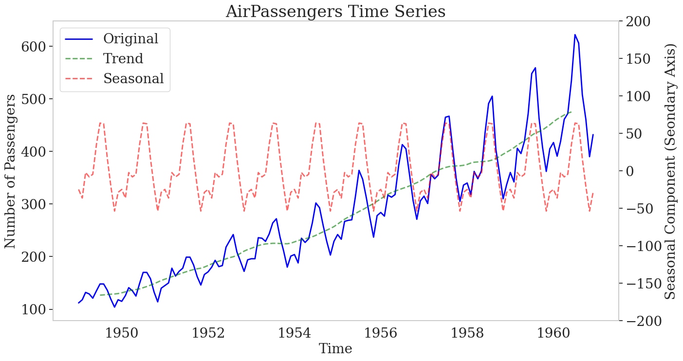
AirPassengers Time Series (1949-1960): This plot illustrates the monthly number of passengers on a US airline from 1949 to 1960. The blue line represents the original data, showing an increasing trend in air travel over the period. The green dashed line indicates the trend component, while the red dashed line depicts the seasonal component, highlighting the recurring patterns in passenger numbers across different months.
In addition to standard descriptive statistical measures of central tendency (mean, median, mode) and variance, time series is defined by its temporal dependence. Temporal dependence is measured through auto-correlation and partial auto-correlation, which help identify the relationships between data points over time and are essential for understanding patterns and making accurate forecasts.
Auto-Correlation and Partial Auto-Correlation
Auto-correlation and partial auto-correlation are statistical measures used in time series analysis to understand the relationship between data points in a sequence.
- Auto-correlation measures the similarity between a data point and its lagged versions. It quantifies the correlation between a data point and previous data points in the sequence. Auto-correlation helps identify patterns and dependencies in the data over time and is often visualized using a correlogram, a plot of the correlation coefficients against the lag.
- Partial auto-correlation measures the correlation between a data point and its lagged versions while controlling for the influence of intermediate data points. It identifies the direct relationship between a data point and its lagged versions, excluding the indirect relationships mediated by other data points. Partial auto-correlation is also visualized using a correlogram.
Both auto-correlation and partial auto-correlation are useful in time series analysis for several reasons:
- Identifying seasonality: Auto-correlation can help detect repeating patterns or seasonality in the data. Significant correlation at a specific lag suggests the data exhibits a repeating pattern at that interval.
- Model selection: Auto-correlation and partial auto-correlation guide the selection of appropriate models for time series forecasting. By analyzing the patterns in the correlogram, you can determine the order of autoregressive (AR) and moving average (MA) components in models like ARIMA (AutoRegressive Integrated Moving Average).
White Noise
Time series that show no autocorrelation are called white noise [1]. In other words, the values in a white noise series are independent and identically distributed (i.i.d.), with no predictable pattern or structure. A white noise series has the following properties:
- Zero mean: The average of the series is zero.
- Constant variance: The variance of the series remains the same over time.
- No auto-correlation: The auto-correlation at any lag is zero, indicating no predictable relationship between the data points.
White noise is crucial in validating the effectiveness of time series models. If the residuals from a model are not white noise, it suggests that there are patterns left in the data that the model has not captured, indicating the need for a more complex or different model.
Seasonality and Cycles
Seasonality refers to the regular patterns or fluctuations in time series data that occur at fixed intervals within a year, such as daily, weekly, monthly, or quarterly. Seasonality is often caused by external factors like weather, holidays, or economic cycles. Seasonal patterns tend to repeat consistently over time.
How To Identify Seasonality in Time-Series Models
Seasonality in time series can be identified by analyzing ACF plots:
- Periodic peaks: Observing peaks in the ACF plot at regular intervals indicates a seasonal lag. For instance, when analyzing monthly data for yearly seasonality, peaks typically appear at lags 12, 24, 36, and so on. Similarly, quarterly data would show peaks at lags 4, 8, 12, etc.
- Significant peaks: Assessing the magnitude of auto-correlation coefficients at seasonal lags helps identify strong seasonal patterns. Higher peaks at seasonal lags compared to others suggest significant seasonality in the data.
- Repetitive patterns: Checking for repetitive patterns in the ACF plot aligned with the seasonal frequency reveals periodicity. Seasonal trends often exhibit repeated patterns of auto-correlation coefficients at seasonal lags.
- Alternating positive and negative correlations: Occasionally, observing alternating positive and negative auto-correlation coefficients at seasonal lags indicates a seasonal pattern.
- Partial Auto-correlation Function (PACF): Complementing the analysis with PACF helps pinpoint the direct influence of a lag on the current observation, excluding indirect effects through shorter lags. Significant spikes in PACF at seasonal lags further confirm seasonality in the data.
By carefully examining the ACF/PACF plot for these indicators, one can infer the presence of seasonal trends in time series data. Additionally, spectral analysis and decomposition methods (e.g., STL decomposition) can also be used to identify and separate seasonal components from the data. This understanding is crucial for selecting appropriate forecasting models and devising strategies to manage seasonality effectively.
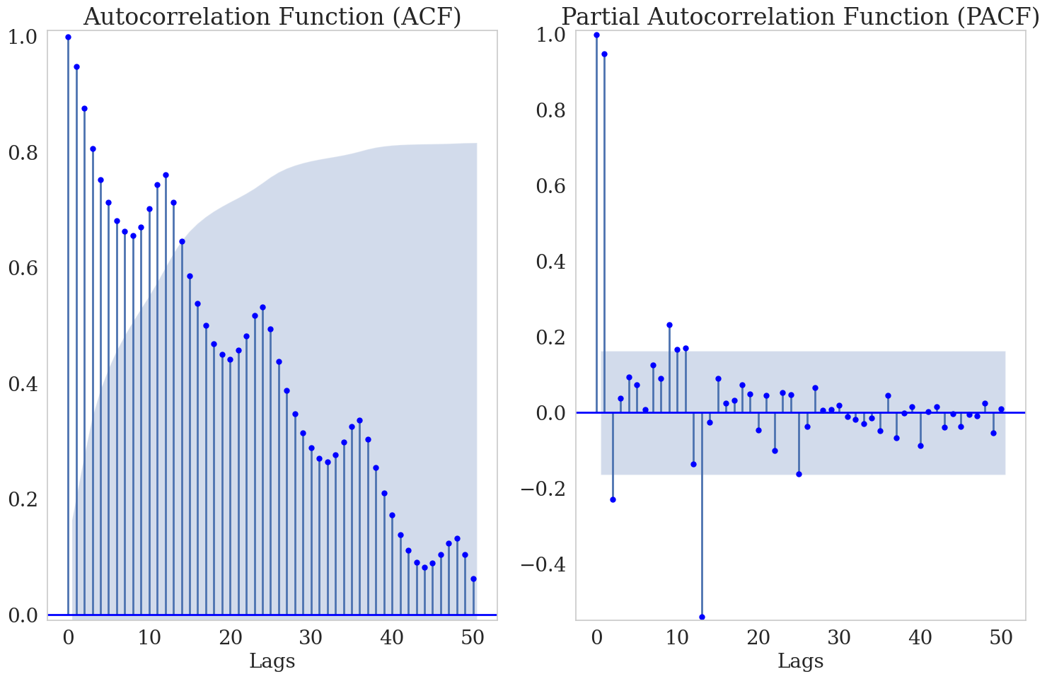
ACF and PACF for AirPassenger Time Series: The plots above show the ACF and PACF correlograms for the airline passenger data. The ACF displays high values for the first few lags, which gradually decrease while remaining significant for many lags. This indicates a strong autocorrelation in the data, suggesting that past values have a significant influence on future values. In the PACF plot, significant peaks occur at lags 12, 24, etc., indicating a yearly seasonality effect in the data.
Cycles, on the other hand, refer to fluctuations in a time series that are not of fixed frequency or period. They are typically longer-term patterns, often spanning several years, and are not as precisely defined as seasonal patterns. Cycles can be influenced by economic factors, business cycles, or other structural changes in the data.
In summary, while both seasonality and cycles involve patterns of variation in time series data, seasonality repeats at fixed intervals within a year. In contrast, cycles represent longer-term fluctuations that may not have fixed periodicity.
Stationarity
Stationarity in time series data implies that statistical characteristics, such as mean, variance, and covariance, remain consistent over time. This stability is crucial for various time-series modeling techniques as it simplifies the underlying dynamics, facilitating accurate analysis, modeling, and forecasting. There are two primary types of stationarity:
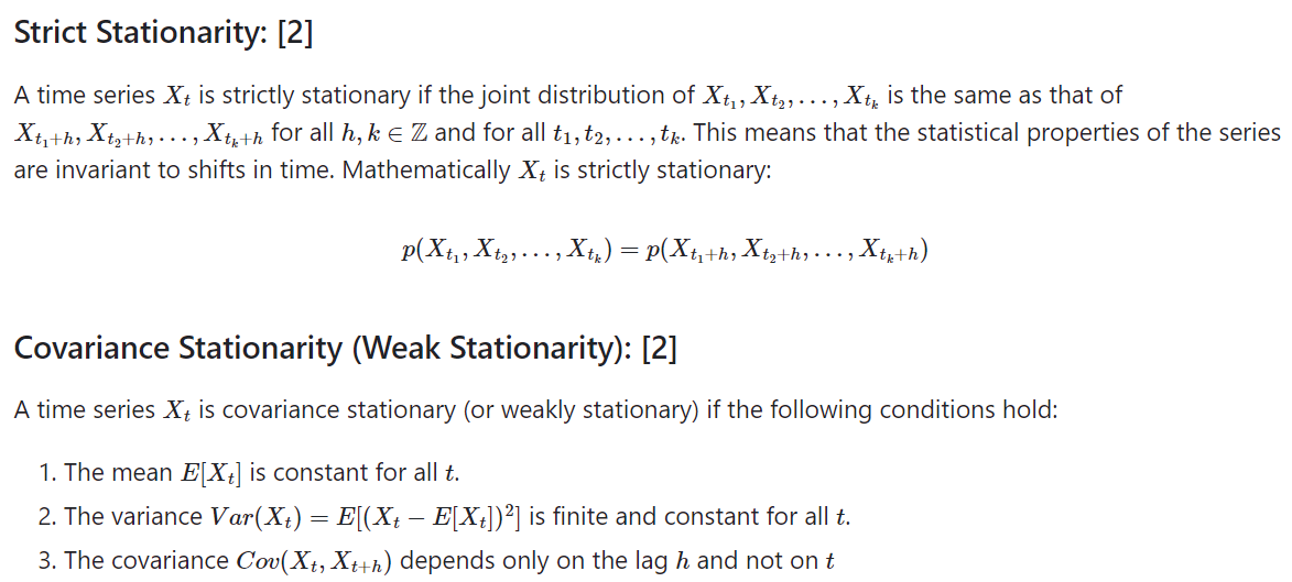
Stationarity is a key concept in time series analysis, as many statistical models assume the data's properties do not change over time. Non-stationary data can lead to unreliable forecasts and spurious relationships, making it crucial to achieve stationarity before modelling.
Why Is Stationarity Important?
Non-stationary time series can be problematic for several reasons:
- Difficulty in modeling: Non-stationary time series violates the assumptions of many statistical models, making it challenging to model and forecast future values accurately. Models like ARIMA (AutoRegressive Integrated Moving Average) assume stationarity, so non-stationary data can lead to unreliable predictions.
- Spurious regression: Non-stationary time series can result in spurious regression, where two unrelated variables appear to be strongly correlated. This can lead to misleading conclusions and inaccurate interpretations of the relationship between variables.
- Inefficient parameter estimation: Non-stationary time series can lead to inefficient parameter estimation. The estimates of model parameters may have large standard errors, reducing the precision and reliability of the estimated coefficients.
Dickey-Fuller Test and Augmented Dickey-Fuller Test
The Dickey-Fuller Test and the Augmented Dickey-Fuller Test are statistical tests used to determine if a time series dataset is stationary or not. They test for the presence of a unit root, which indicates non-stationarity. A unit root suggests that shocks to the time series have a permanent effect, meaning the series does not revert to a long-term mean.
- Limitations: These tests can be sensitive to the choice of lag length and may have low power in small samples. It's essential to interpret the results alongside other diagnostic checks carefully.
| ADF Test on AirPassengers Time series | Test Result |
|---|---|
|
Python
|
ADF Statistic 0.815 p-value 0.992 Critical Values (1%) -3.482 Critical Values (5%) -2.884 Critical Values (10%) -2.579 Given the high p-value (0.992) and the fact that ADF statistic (0.815) is greater than the critical values, we fail to reject the null hypothesis. Therefore, there is strong evidence to suggest that the time series is non-stationary and possesses a unit root. |
How To Make a Time Series Stationary if It Is Not Stationary
- Differencing: For example, First-Order Differencing involves subtracting the previous observation from the current observation. If the time series has seasonality, seasonal differencing can be applied.
- Transformations: Techniques like logarithm, square root, or Box-Cox can stabilize the variance.
- Decomposition: Decomposing the time series into trend, seasonal, and residual components.
- Detrending: For instance, subtracting the Rolling Mean or fitting and removing a Linear Trend.
It is important to identify and address non-stationarity in time series analysis to ensure reliable and accurate modeling and forecasting.
Modeling Univariate Time Series
Wold Representation Theorem
The Wold decomposition theorem states that any covariance stationary process can be decomposed into two mutually uncorrelated components. The first component is a linear combination of past values of a white noise process, while the second component consists of a process whose future values can be precisely predicted by a linear function of past observations.

The Wold theorem is fundamental in time series analysis, providing a framework for understanding and modelling stationary time series.
Lag Operator
The lag operator (L) helps to succinctly represent the differencing operations. It shifts a time series back by a one-time increment.
Exponential Smoothing
Exponential smoothing is a time series forecasting technique that applies weighted averages to past observations, giving more weight to recent observations while exponentially decreasing the weight for older observations. This method is useful for making short-term forecasts and smoothing out irregularities in the data.
Simple Exponential Smoothing
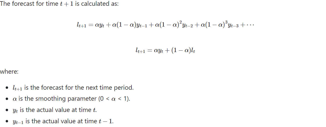
Simple exponential smoothing is a technique where the forecast for the next period is calculated as a weighted average of the current period's observation and the previous prediction. This technique is suitable for time series data without trend or seasonality.
ARMA (AutoRegressive Moving Average) Model
The ARMA model is a popular time series model that combines both autoregressive (AR) and moving average (MA) components. It is used to forecast future values of a time series based on its past values.
The autoregressive (AR) component of the ARMA model represents the linear relationship between the current observation and a certain number of lagged observations. It assumes that the current value of the time series is a linear combination of its past values. The order of the autoregressive component, denoted by p, determines the number of lagged observations included in the model.
The moving average (MA) component of the ARMA model represents the linear relationship between the current observation and a certain number of lagged forecast errors. It assumes that the current value of the time series is a linear combination of the forecast errors from previous observations. The order of the moving average component, denoted by q, determines the number of lagged forecast errors included in the model.
The ARMA model can be represented by the following equation:
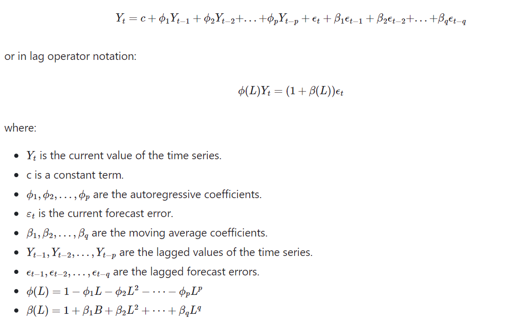
The ARMA model can be estimated using various methods, such as maximum likelihood estimation or least squares estimation.
ARIMA Model
ARIMA includes an integration term, denoted as the "I" in ARIMA, which accounts for non-stationarity in the data. ARIMA models handle non-stationary data by differencing the series to achieve stationarity.
In ARIMA models, the integration order (denoted as "d") specifies how many times differencing is required to achieve stationarity. This is a parameter that needs to be determined or estimated from the data. ARMA models do not involve this integration order parameter since they assume stationary data.

SARIMA Model
SARIMA stands for Seasonal AutoRegressive Integrated Moving Average. It is an extension of the ARIMA model that incorporates seasonality into the modelling process. SARIMA models are particularly useful when dealing with time series data that exhibit seasonal patterns.
SARMIAX
The SARIMAX model is defined by the parameters (p, d, q) and (P, D, Q, s):
- (p, d, q): These are the non-seasonal parameters.
- p: The order of the non-seasonal AutoRegressive (AR) part
- d: The number of non-seasonal differences needed to make the series stationary
- q: The order of the non-seasonal Moving Average (MA) part
- (P, D, Q, s): These are the seasonal parameters.
- P: The order of the seasonal AutoRegressive (AR) part.
- D: The number of seasonal differences needed to make the series stationary.
- Q: The order of the seasonal Moving Average (MA) part.
- s: The length of the seasonal cycle (e.g., s=12 for monthly data with yearly seasonality).
- Exogenous Variables (X): These are external variables that can influence the time series but are not part of the series itself. For example, economic indicators or weather data might be included as exogenous variables.
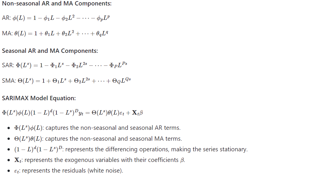
SARIMAX Model For Air Passenger Time Series
To identify the optimal order of a Seasonal AutoRegressive Integrated Moving Average (SARIMA) model, the auto_arima function from the pmdarima [4] library was utilized. It automates the identification of optimal parameters for the SARIMAX model.
Sarimax_model = auto_arima(train_data,
                           start_p=0, start_q=0,
                           max_p=6, max_q=6,
                           max_d=12,
                           seasonal=True,
                           m=12,  # Seasonal period (e.g., 12 for monthly data with yearly seasonality)
                           start_P=0, start_Q=0,
                           max_P=25, max_Q=25,
                           d=None, D=None,
                           max_D=25,
                           trace=True,
                           error_action='ignore',
                           suppress_warnings=True,
                           stepwise=True,
                           random = True,
                           n_fits = 10,
                           information_criterion = 'aic')
Sarimax_model.summary()
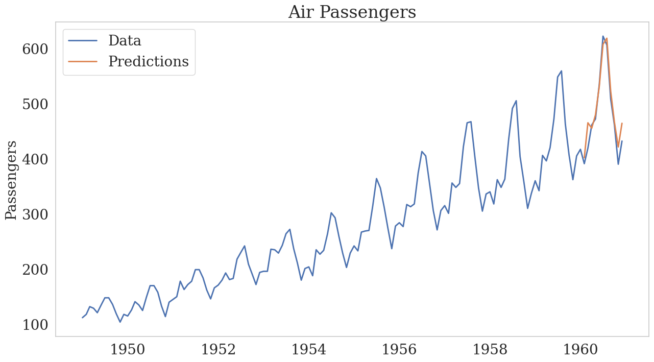
As per the auto_arima grid search, the optimal order for model is: SARIMAX(1, 1, 0)x(0, 1, 0, 12).
Modeling Volatility
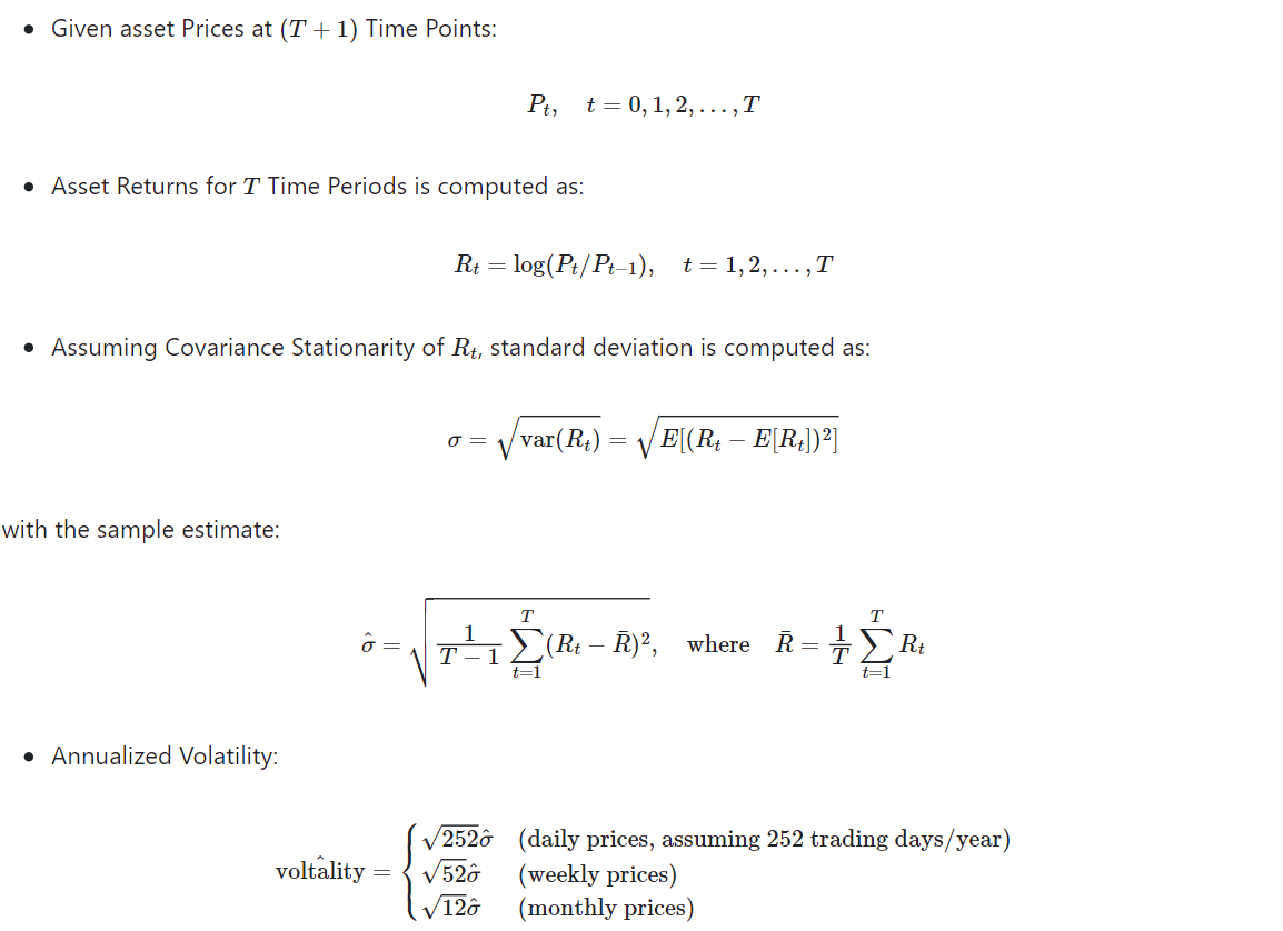
The volatility of a time series refers to the degree of variation or dispersion in the series over time. It is a measure of how much the series deviates from its average or expected value. Volatility is particularly relevant in financial markets but can also apply to other types of time series data where variability is important to understand or predict. It is often measured as the annualized standard deviation change in price or value of financial security; e.g., for asset price volatility, which is computed as follows [2]:
Simple Methods to Model Volatility
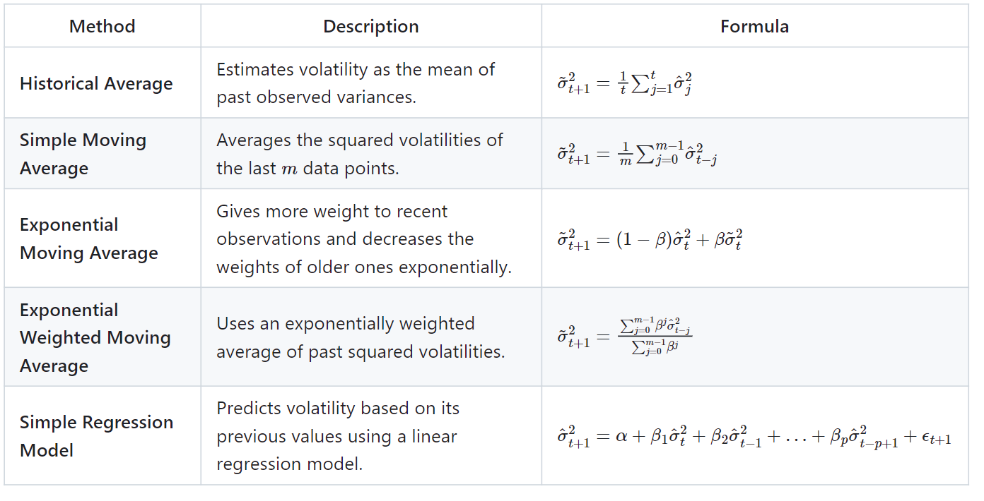
ARCH (Autoregressive Conditional Heteroskedasticity) Model
ARCH models are a class of models used in econometrics and financial econometrics to analyze time series data, particularly in the context of volatility clustering. These models are designed to capture the time-varying volatility or heteroskedasticity in financial time series data, where the volatility of the series may change over time.
In statistics, a sequence of random variables is homoscedastic if all its random variables have the same finite variance; this is also known as homogeneity of variance. The complementary notion is called heteroscedasticity, also known as heterogeneity of variance [3].
The basic idea behind ARCH models is that the variance of a time series can be modeled as a function of its past values, along with possibly some exogenous variables. In other words, the variance at any given time is conditional on the past observations of the series.
- ARCH (1) model derivation:
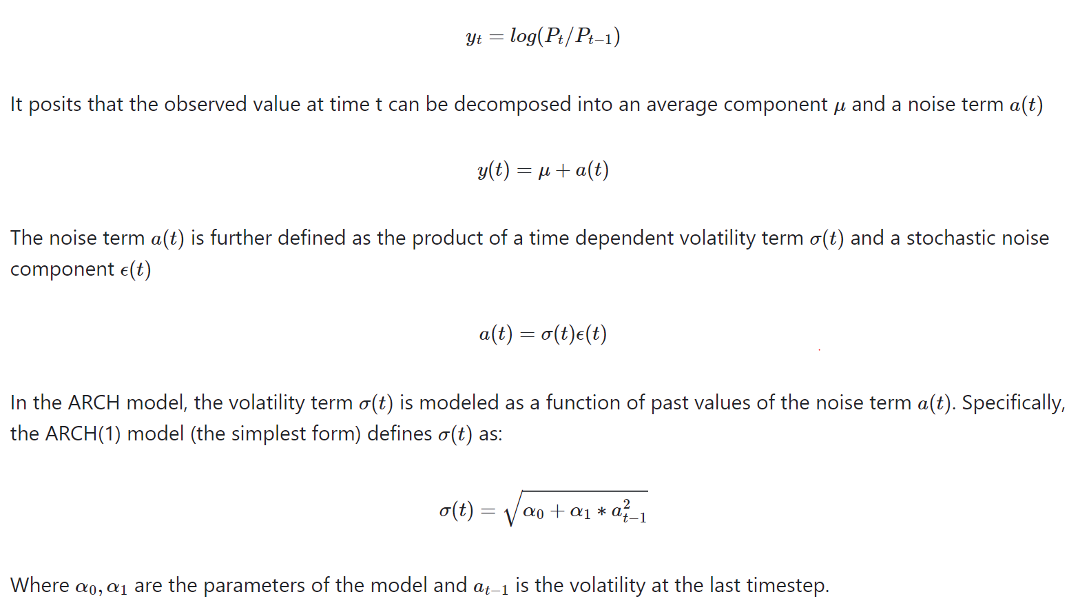
- ARCH (p) model:

GARCH (Generalized Autoregressive Conditional Heteroskedasticity) Model
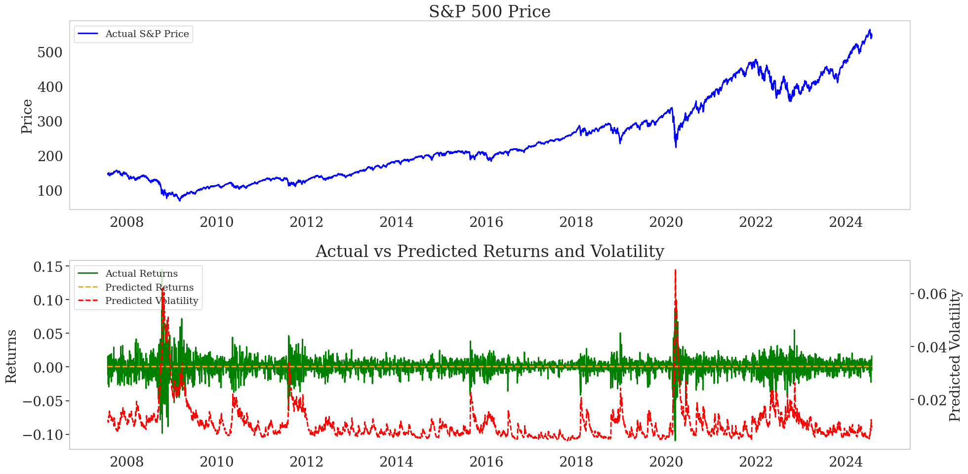
The GARCH model is an extension of the ARCH Model. It models time series as a function of previous values as well as volatility.
GARCH for S&P 500 volatility:
Review: ARMA and GARCH
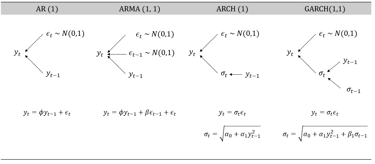
- AR/ARMA models: Best suited for stationary time series data, where statistical properties like mean and variance are constant over time; Useful for short-term forecasting, ARMA models combine both autoregressive (AR) and moving average (MA) components to capture the dynamics influenced by past values and past forecast errors.
- AR models: Used when the primary relationship in the data is between the current value and its past values; Suitable for time series where residuals show no significant autocorrelation pattern, indicating that past values alone sufficiently explain the current observations.
- ARMA models: Employed when both past values and past forecast errors significantly influence the current value; This combination provides a more comprehensive model for capturing complex dynamics in time series data.
- ARCH models: Best suited for time series data with volatility clustering but lacking long-term persistence; ARCH models capture bursts of high and low volatility effectively by modelling changing variance over time based on past errors.
- GARCH models: Extend ARCH models by incorporating past variances, allowing them to handle more persistent volatility; GARCH models are better at capturing long-term dependencies in financial time series data, making them suitable for series with sustained periods of high or low volatility.
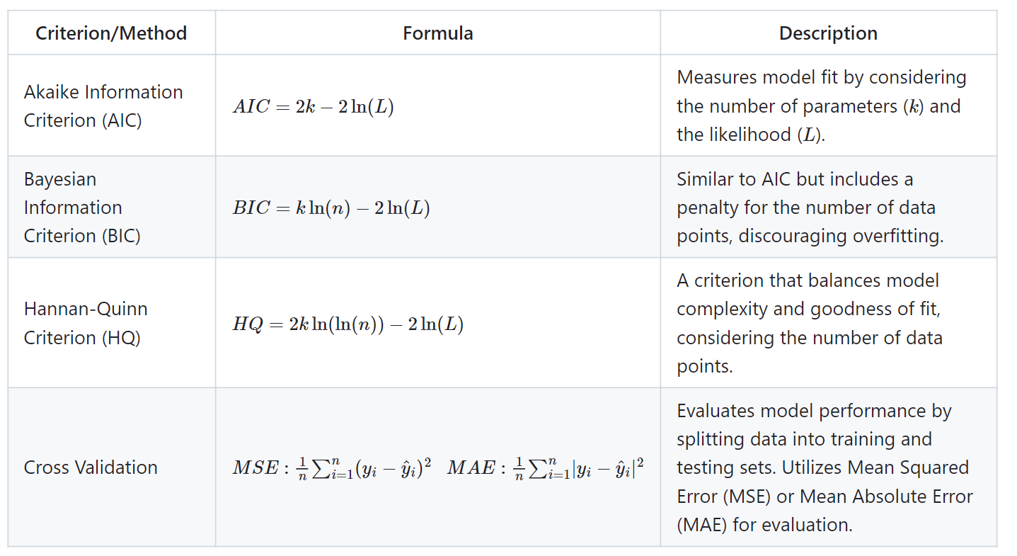
Model Selection
When analyzing time series data, selecting the appropriate model (e.g., AR vs ARMA) and determining the model's order is crucial for making accurate predictions. Several methods can be used for model selection:
Conclusion
Time series analysis is a critical tool for understanding and predicting temporal data patterns across various fields, from finance and economics to healthcare and climate science. A solid grasp of classical time series models, such as ARMA, ARIMA, SARIMA, ARCH, and GARCH, alongside fundamental concepts like stationarity, auto-correlation, and seasonality, is crucial for developing and fine-tuning more advanced methodologies. Classical models provide foundational insights into time series behavior, guiding the application of more sophisticated techniques. Mastery of these basics not only enhances understanding of complex models but also ensures that forecasting methods are robust and reliable.
By leveraging the principles and performance benchmarks established through classical models, practitioners can optimize advanced approaches, such as machine learning algorithms, deep learning, and hybrid models, leading to more accurate predictions and better-informed decision-making.
References
[1] Hyndman, R.J., & Athanasopoulos, G. (2021) Forecasting: principles and practice, 3rd edition, OTexts: Melbourne, Australia. Accessed on June 15, 2024.
[2] MIT, Topics in mathematics with application in finance.
[3] Homoscedasticity and heteroscedasticity. Accessed on June 29, 2024.
Opinions expressed by DZone contributors are their own.

Comments