Performance Ingredients for NoSQL: Intersect Scans in N1QL
Query processing is one of the most complex and complicated areas in the database realm. Intersect scans leverage multiple indexes for a query and bring subtle performance characteristics.
Join the DZone community and get the full member experience.
Join For FreeCouchbase Server N1QL Query Engine is SQL for JSON
It’s not an exaggeration to say that query processing has produced tons of papers and patents. It is one of the most complex and complicated areas in the database realm. With the proliferation of NoSQL/document databases and more adoption into the enterprise, there is high demand and a requirement for sophisticated query processing capabilities for NoSQL beyond k/v get/set accesses. Remember, the JSON data model is the foundation of document databases that brings the most value to NoSQL (among others like scale-out, HA, and performance) with its fundamentally different capabilities (w.r.t RDBMS) such as flexible schema and hierarchical and multi-valued data.
In this blog, I will try to explain some of the performance ingredients and optimization techniques used for efficient JSON query processing. More specifically, I will cover intersect scans, which leverages multiple indexes for a query and brings subtle performance characteristics. For simplicity, I will use the latest Couchbase Server 4.6 N1QL engine and the packaged travel-sample data for examples. Note that N1QL is the most sophisticated query engine and the most comprehensive implementation of SQL (in fact, SQL++) for JSON data model.
Fundamentals of Performance
The performance of any system follows physics. The basic two rules can be (loosely) stated as:
Quantity: Less work is more performance.
Quality: Faster work is more performance.
Query processing is no different and it also tries to optimize both these factors in various forms and scenarios to bring efficiency. Each optimization is different and results in a different amount of performance benefit. As the saying goes, every nickel adds to a dollar, and the N1QL engine keeps incorporating performance enhancements to run queries as efficiently as possible.
Intersect Scans: Using Multiple Indexes for AND Queries
As you might already know, secondary indexes (just "indexes" for short) are the biggest performance techniques used by query processing. Database indexes help with efficiently mapping and finding document attributes to documents. For example, with user profile employee documents, a key-value store can fetch a particular document only if the corresponding document_key is available. However, creating an index on the name attribute of the document maintains mapping of all name values to the set of documents holding a specific name value. This is called index-lookup or IndexScan operation.
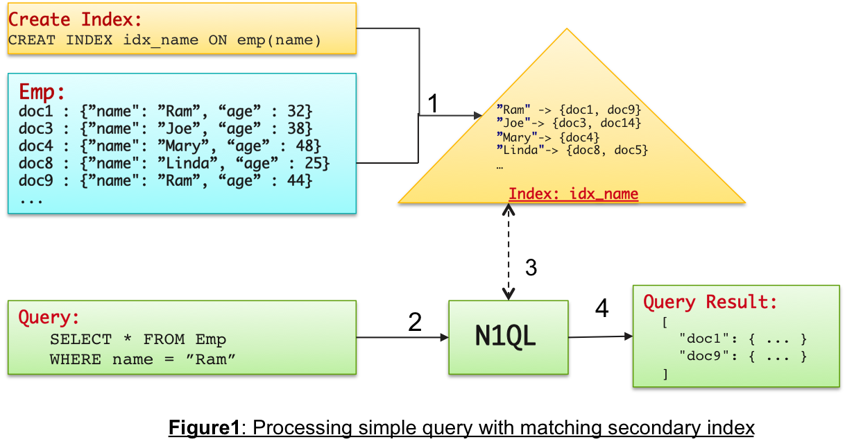
When one index satisfies lookup for a query predicate, it is called a simple IndexScan. However, when a query has multiple AND predicate conditions, then different available indexes may satisfy different conditions in the WHERE-clause. In such case, N1QL uses the technique called Intersect Scan, where both the indexes are used to find documents matching the predicates. The technique is based on the premise that the intersection of the sets of documents obtained by IndexScan lookups from each of the satisfying indexes is equal to the logical-AND of applying respective individual predicates. Note that this is related, but very different from using composite indexes, where a single index is created on multiple fields used in different predicates of the query. Will cover it later in the blog.
Let’s understand this with some simpler example. Consider following query which has predicates on name and age , and also assume we have two indexes created on the two fields used in the WHERE-clause.
CREATE INDEX idx_name ON emp(name);
CREATE INDEX idx_age ON emp(age);
SELECT * FROM emp WHERE name = “Ram” and age < 35;
In this case, both the indexes can satisfy the query predicate, but neither can fully help the two predicate conditions. By using simple IndexScan, the N1QL query engine can do following:
Use the
nameindex idx_name:In this case, index idx_name is looked up to first find all the documents keys which match
name = “Ram”.Then, respective documents are fetched and the second filter
age < 35is appliedFinally, query returns the set of documents which matched both the filers.
Use the
ageindex idx_age.In this case, the index idx_age is looked up first, to find all the document keys which match
age < 35.Then, respective documents are fetched and the second filter
name = “Ram”is applied.Finally, the query returns the set of documents which matched both the filers.
Both approaches make sense and produce correct results. However, they have very significant and subtle performance characteristics. The performance depends on a property called selectivity of the predicate conditions, which is defined as the ratio of the number of documents matching particular predicate to the total number of documents considered. For instance:
If the there 100 documents in the
empbucket and five employees have name "Ram," then the selectivity of the predicate(name = ‘Ram’)is 5/100 = 0.05 (or 5% for simplicity).Similarly, if 40% of the 100 employees are aged less than 35, then the selectivity of
(age < 35)is 0.4.Finally, the selectivity of the conjunctive predicate will be <= min(0.05, 0.4).
Now you might be wondering what these selectivities have anything to do with the query performance. Let’s connect the dots by looking at the two IndexScan approaches we talked above:
Use the
nameindex idx_name.Index lookup finds five documents matching
(name = ‘Ram’)and returns the corresponding document keys to N1QL.The five documents are fetched, and second filter
(age < 35)is applied. Assume two documents satisfy this condition (i.e., selectivity of both predicates together is 0.02 or 2%).The two documents matching both the filters are returned as the final result.
Use the
ageindex idx_age.Index lookup finds 40 documents matching
(age < 35)and returns the corresponding 40 document keys to N1QL.The 40 documents are fetched, and second filter
(name = ‘Ram’)is applied. Only two documents will satisfy this condition.The two documents matching both the filters are returned as the final result.
Now, it’s very apparent that the first approach using the index idx_name is much more efficient than the second approach of using idx_age. The first approach is doing less work in each of the steps. In particular, fetching five documents instead of 40 is huge!
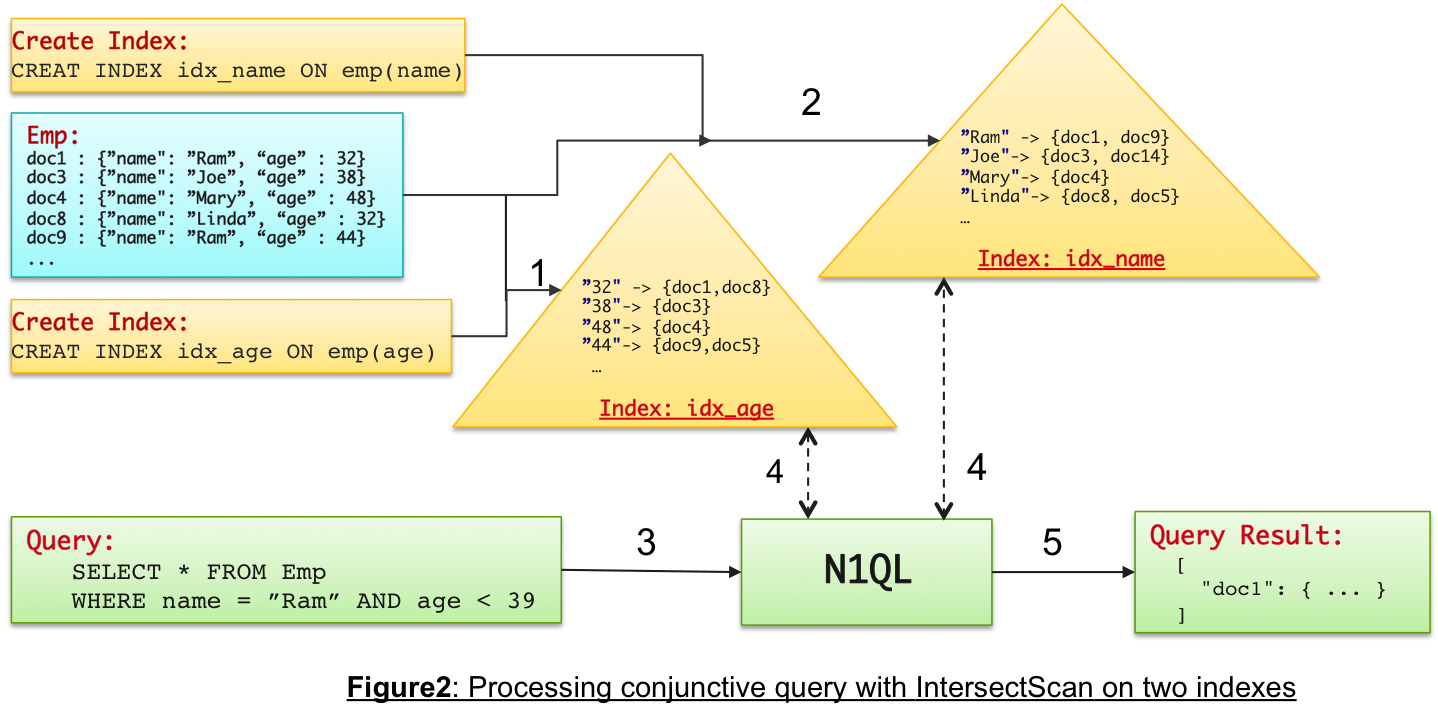
We can generalize this and say it is always efficient to evaluate predicates with lower selectivity values, followed by higher selectivities. Relational databases understand these factors very well, and their cost-based query optimizers maintain enough statistics to figure the best index for the query. N1QL is a rule-based query optimizer and solves this problem smartly using Intersect Scans to both the indexes. The steps are:
Send parallel request to both indexes with respective predicates.
Index lookup of idx_name with (name = ‘Ram’), which returns five document keys.
Index lookup of idx_age with (age < 35), which returns 40 document keys.
The intersection of the two sets of the keys is performed, which returns the two document keys that should satisfy both the filters.
The two documents are fetched, predicates are reapplied (to cover any potential inconsistencies between index and data), and final results are returned. Note that, for performance reasons, indexes are maintained asynchronously to reflect any data or document changes. N1QL provides various consistency levels that can be specified per query.
Performance Characteristics of IntersectScan
The following observations can be made from the above five steps of how IntersectScan's work:
IntersectScan can be more performant when the final result of the conjunctive predicate is much smaller than that of individual filters.
IntersectScan does index lookups to all satisfying indexes. This may be unnecessary, for example, when we know a specific index is best, or when some index lookups don't filter any documents (such as duplicate indexes, or when an index is subset of another). So, when we have a lot of satisfying indexes, InterSect scans can be more expensive (than using a specific index).
- The Subset of satisfying indexes can be provided to the query using the USE INDEX (idx1, idx2, ...) clause, to override N1QL default behavior of picking all satisfying indexes for the IntersectScan.
- As there are pros and cons of using IntersectScans, always check the EXPLAIN output of your performance sensitive queries and make sure if the IntersectScans are used appropriately.
Look at my blog on N1QL performance improvements in Couchbase Server 4.6 release for few such subtle optimizations related to IntersectScans.
Comparing With Composite Indexes: Flexibility vs. Performance
As it is clear by now, the purpose of IntersectScans is to efficiently run queries with conjunctive queries. Composite indexes are an excellent alternative to doing the same, and yes, there are trade-offs. A composite index is an index with multiple fields as index-keys. For example, the following index is created with name andage:
CREATE INDEX idx_name_age ON emp(name, age);This index can very well fully satisfy the query discussed earlier and perform as well as (or slightly better) than the IntersectScan. However, this index cannot help a query with a filter on just age field, such as:
Q1: SELECT * FROM emp WHERE age = 35That will violate the prefix-match constraint of the composite indexes. That means that to use a composite index, all the prefixing index-keys/fields must be specified as part of the WHERE-clause. In this example, name must be used in the WHERE-clause to be able to use the index idx_name_age. as in:
Q2: SELECT * FROM emp WHERE age = 35 AND name IS NOT MISSING;There are two problems with this rewritten query Q2:
Q2 is not equivalent to Q1. For example, Q1 may return more documents which has a missing
namefield.The selectivity of the spurious predicate
(name IS NOT MISSING)may be really high, thus pretty much converting the indexScan into a full scan. That means the index lookup will go through all index entries which have non-missingname, and then subsequently check for(age = 35). In contrast, when using the index idx_age, the index entry for(age = 35)is a straight point-lookup and returned instantaneously.
Further, it is important to understand that the size of the composite index gets larger with the number of index keys. Lookups/scans on a bigger index will be more expensive, than those on a smaller index (on one field). To summarize:
Composite indexes are a better choice to optimize specific queries.
Simple indexes (on one or more fields), along with IntersectScans are a better choice for ad hoc queries which need the flexibility of conjunctive predicates on various fields.
Example
Let’s look at a live example with travel-sample data and precreated indexes def_type and def_sourceairport shipped with the product. Ran these tests with Couchbase Server 4.6 DP release on my Mac Pro laptop. The query finds the destination airports and number of stops/hops, starting from SFO.
Use the index def_type:
EXPLAIN SELECT destinationairport, stops
FROM `travel-sample`
USE INDEX (def_type)
WHERE type = "route" AND sourceairport = "SFO";
[
  {
    "plan": {
      "#operator": "Sequence",
      "~children": [
        {
          "#operator": "IndexScan",
          "index": "def_type",
          "index_id": "e23b6a21e21f6f2",
          "keyspace": "travel-sample",
          "namespace": "default",
          "spans": [
            {
              "Range": {
                "High": [
                  "\"route\""
                ],
                "Inclusion": 3,
                "Low": [
                  "\"route\""
                ]
              }
            }
          ],
          "using": "gsi"
        },
        {
          "#operator": "Fetch",
          "keyspace": "travel-sample",
          "namespace": "default"
        },
        {
          "#operator": "Parallel",
          "~child": {
            "#operator": "Sequence",
            "~children": [
              {
                "#operator": "Filter",
                "condition": "(((`travel-sample`.`type`) = \"route\") and ((`travel-sample`.`sourceairport`) = \"SFO\"))"
              },
              {
                "#operator": "InitialProject",
                "result_terms": [
                  {
                    "expr": "(`travel-sample`.`destinationairport`)"
                  },
                  {
                    "expr": "(`travel-sample`.`stops`)"
                  }
                ]
              },
              {
                "#operator": "FinalProject"
              }
            ]
          }
        }
      ]
    },
    "text": "SELECT destinationairport, stops\nFROM `travel-sample`\nUSE INDEX (def_type) \nWHERE type = \"route\" AND sourceairport = \"SFO\";"
  }
]
This query took on average 650msec. Note that the selectivity of (type = 'route') is 0.76 (i.e., 24,024 of 31,592 docs).
SELECT (SELECT RAW count(*) FROM `travel-sample` t where type = "route")[0]/
       (SELECT RAW count(*) FROM `travel-sample` t1)[0] as selectivity;
[
  {
    "selectivity": 0.7604456824512534
  }
]
Similarly, the selectivity of (sourceairport = 'SFO') is ~0.0079 (i.e., 249 of 31,592 docs).
SELECT (SELECT RAW count(*) FROM `travel-sample` t where sourceairport = "SFO")[0]/
       (SELECT RAW count(*) FROM `travel-sample` t1)[0]  as selectivity;
[
  {
    "selectivity": 0.007881742213218537
  }
]
Hence, using the index def_sourceairport should be much more efficient.
Use the index def_sourceairport:
EXPLAIN SELECT destinationairport, stops
FROM `travel-sample`
USE INDEX (def_sourceairport)
WHERE type = "route" AND sourceairport = "SFO";
[
  {
    "plan": {
      "#operator": "Sequence",
      "~children": [
        {
          "#operator": "IndexScan",
          "index": "def_sourceairport",
          "index_id": "c36ffb6c9739dcc9",
          "keyspace": "travel-sample",
          "namespace": "default",
          "spans": [
            {
              "Range": {
                "High": [
                  "\"SFO\""
                ],
                "Inclusion": 3,
                "Low": [
                  "\"SFO\""
                ]
              }
            }
          ],
          "using": "gsi"
        },
        {
          "#operator": "Fetch",
          "keyspace": "travel-sample",
          "namespace": "default"
        },
        {
          "#operator": "Parallel",
          "~child": {
            "#operator": "Sequence",
            "~children": [
              {
                "#operator": "Filter",
                "condition": "(((`travel-sample`.`type`) = \"route\") and ((`travel-sample`.`sourceairport`) = \"SFO\"))"
              },
              {
                "#operator": "InitialProject",
                "result_terms": [
                  {
                    "expr": "(`travel-sample`.`destinationairport`)"
                  },
                  {
                    "expr": "(`travel-sample`.`stops`)"
                  }
                ]
              },
              {
                "#operator": "FinalProject"
              }
            ]
          }
        }
      ]
    },
    "text": "SELECT destinationairport, stops\nFROM `travel-sample`\nUSE INDEX (def_sourceairport) \nWHERE type = \"route\" AND sourceairport = \"SFO\";"
  }
]
As expected, this query ran much more efficiently, and took (on average) 18msec.
If no specific index is used (or multiple indexes are specified), N1QL does IntersectScan with all available satisfying indexes:
EXPLAIN SELECT destinationairport, stops
FROM `travel-sample`
USE INDEX (def_sourceairport, def_type)
WHERE type = "route" AND sourceairport = "SFO";
[
  {
    "plan": {
      "#operator": "Sequence",
      "~children": [
        {
          "#operator": "IntersectScan",
          "scans": [
            {
              "#operator": "IndexScan",
              "index": "def_type",
              "index_id": "e23b6a21e21f6f2",
              "keyspace": "travel-sample",
              "namespace": "default",
              "spans": [
                {
                  "Range": {
                    "High": [
                      "\"route\""
                    ],
                    "Inclusion": 3,
                    "Low": [
                      "\"route\""
                    ]
                  }
                }
              ],
              "using": "gsi"
            },
            {
              "#operator": "IndexScan",
              "index": "def_sourceairport",
              "index_id": "c36ffb6c9739dcc9",
              "keyspace": "travel-sample",
              "namespace": "default",
              "spans": [
                {
                  "Range": {
                    "High": [
                      "\"SFO\""
                    ],
                    "Inclusion": 3,
                    "Low": [
                      "\"SFO\""
                    ]
                  }
                }
              ],
              "using": "gsi"
            }
          ]
        },
        {
          "#operator": "Fetch",
          "keyspace": "travel-sample",
          "namespace": "default"
        },
        {
          "#operator": "Parallel",
          "~child": {
            "#operator": "Sequence",
            "~children": [
              {
                "#operator": "Filter",
                "condition": "(((`travel-sample`.`type`) = \"route\") and ((`travel-sample`.`sourceairport`) = \"SFO\"))"
              },
              {
                "#operator": "InitialProject",
                "result_terms": [
                  {
                    "expr": "(`travel-sample`.`destinationairport`)"
                  },
                  {
                    "expr": "(`travel-sample`.`stops`)"
                  }
                ]
              },
              {
                "#operator": "FinalProject"
              }
            ]
          }
        }
      ]
    },
    "text": "SELECT destinationairport, stops\nFROM `travel-sample`\nUSE INDEX (def_sourceairport, def_type) \nWHERE type = \"route\" AND sourceairport = \"SFO\";"
  }
]
This query also ran very efficiently in 20msec.
Summary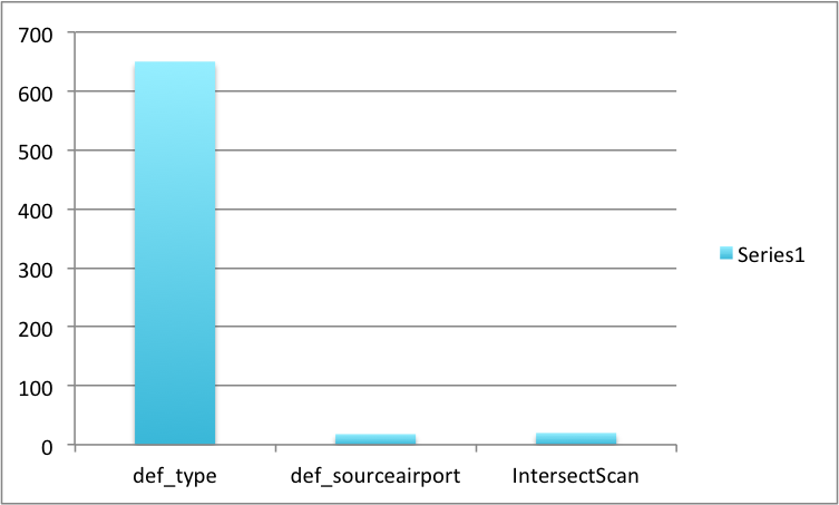
Run times with the individual indexes and IntersectScan are shown in this chart. Note that the latency with the IntersectScan is almost same as that with the index def_sourceairport because the selectivities of the conjunctive predicate is the same as that of (sourceairport = 'SFO'). Basically, the soruceairport field exists only in the type = 'route' documents in travel-sample.
Hope this gives some insights into the intricacies involved in achieving query performance and the interplay between various factors such as the query, predicates, selectivities, and index-type.
Couchbase Server 4.6 Developer Preview is available now. It has a bunch of cool performance optimizations in N1QL. Try it out and let me know any questions, or just how awesome it is.
Opinions expressed by DZone contributors are their own.
Comments