Architecting Petabyte-Scale Hyperspectral Pipelines on AWS

The Data Challenge

Every industry has its version of the same data engineering problem: massive, complex payloads generated at the edge — far from the cloud, often on unreliable networks — that need to become queryable, structured datasets as fast as possible. In genomics, it is multi-gigabyte sequencing files produced by instruments in labs. 

In autonomous vehicles, it is LiDAR and camera telemetry streaming off test fleets. The underlying architectural challenge is the same in every case: ingest heavy data at burst scale, store it cost-effectively for years, and transform it into something an analyst or ML model can actually use without touching the raw files.

This article uses hyperspectral imaging in digital agriculture as the concrete use case, but the architecture is designed to be general-purpose and replicable. Hyperspectral sensors capture light across hundreds of spectral bands, making it possible to detect water stress, nutrient deficiencies, and early disease in crops well before anything is visible to the human eye.

A single sensor pass over a 160-acre field generates 40–80 GB of raw data. These are not images in any conventional sense — they are three-dimensional tensors, often called “hypercubes,” where every spatial pixel carries reflectance measurements across 200 or more contiguous spectral bands. The files arrive in scientific formats like HDF5, NetCDF, or ENVI, which do not support partial reads over a network without specialized tooling. Loading an entire 4 GB cube into memory just to extract a vegetation index from three bands is wasteful at the small scale and operationally unaffordable once a mid-size operation is producing 5–10 TB of raw cubes per growing season.

The architecture described here solves that problem end to end: from raw sensor capture to queryable, structured tables in the cloud with cost-efficient storage and minimal dependency on network bandwidth. The patterns — event-driven ingestion, aggressive storage tiering, medallion lakehouse design, and containerized edge processing — are all portable. Swap the hyperspectral cube in this architecture pattern for a FASTQ file or a LiDAR point cloud, and the same blueprint applies with very minimal modifications.

Ingestion: Handling Seasonal Burst Traffic

Agricultural data arrives in extreme seasonal bursts. During harvest, hundreds of edge nodes may be uploading simultaneously; in winter, the pipeline sits nearly idle. Any architecture that provisions fixed compute for this pattern is going to be very inefficient, so the ingestion layer needs to scale to near-zero in both directions.

The pipeline uses an S3 → SQS → Lambda → Batch pattern, and the SQS queue in the middle is what makes the rest of it work. When files land in S3, event notifications route into the queue, which acts as a buffer between the unpredictable arrival rate and the compute layer downstream. Lightweight Lambda functions essentially like an air traffic controller poll the queue, bundle incoming file references into manifest batches of 50–200 cubes, and submit those manifests to AWS Batch. Batch spins up Spot Instances to do the actual heavy processing.

Triggering Lambda directly from S3 events was the first approach, but it breaks down at scale for two reasons: Lambda’s concurrency limits create a hard ceiling during burst ingest, causing silent throttling and dropped events, and the 1:1 mapping between files and Lambda invocations is inefficient when the processing works much better against batches of files. Putting SQS in the middle solves both problems at once.

When selecting the compute environment, AWS Batch ultimately won out over the alternatives after some evaluation. The main limitation of Fargate was its hard memory ceiling of around 30 GB. This was simply too tight for processing a 4 GB data cube with intermediate arrays in memory that can easily require 32–64 GB of RAM. Batch also provides native handling for job queuing, retries, and Spot interruption recovery. Since the workload is highly parallel and interruption-tolerant, this capability allowed us to safely leverage Spot pricing, delivering a significant 60–90% cost reduction that would have been difficult to justify passing up.

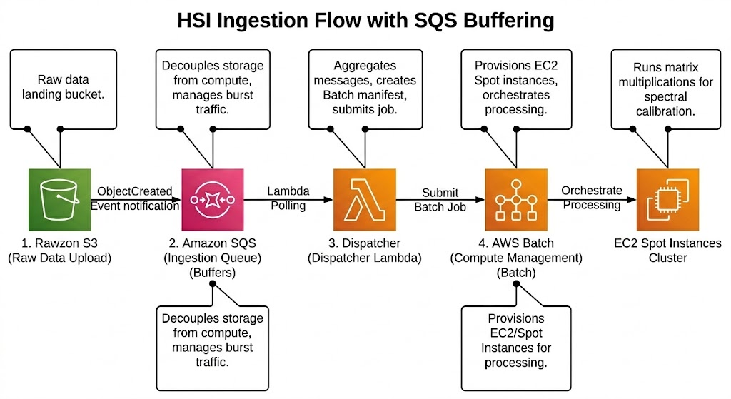
One early lesson involved S3 prefix design. A flat raw/ prefix structure ran into per-prefix request rate limits (3,500 PUTs/second) during burst ingest, which caused throttling that was initially difficult to diagnose. Restructuring to region/farm_id/year/month/day/ spread the writes across thousands of unique prefixes and also aligned neatly with the partition scheme used by Athena and Trino downstream, so the same naming convention solved both the throughput problem and the query performance problem.

Storage: Managing Petabyte-Scale Costs

At this scale, storage costs will quietly become the largest line item in the project if the tiering strategy is not aggressive from day one. Petabytes of data at $0.023/GB/month in S3 Standard add up fast, but deleting raw scientific data is not an option due to regulatory reasons and for future model improvements.

The lifecycle strategy moves successfully processed cubes to Glacier Instant Retrieval within 24 hours. The initial instinct was to go straight to Deep Archive, but in practice, about 5–8% of cubes get retrieved within the first year—sensor calibrations get updated, new vegetation index algorithms need validation against historical data, and so on. Deep Archive’s 12-hour restoration time makes that retrieval workflow painful enough to slow down the R&D cycle. Glacier IR runs at roughly $0.004/GB/month, about 6x cheaper than Standard, with millisecond retrieval. After a year, once retrieval rates drop below 1%, a second lifecycle rule transitions everything to Deep Archive.

The important detail in the lifecycle configuration is a tag-based filter that gates the transition on processing_status = complete. Without this check, cubes that failed processing end up in Glacier, and restoring them for a retry becomes an unnecessary expense that multiplies quickly during periods of high ingest.

# Terraform: Tiered lifecycle for raw HSI cubes
resource "aws_s3_bucket_lifecycle_configuration" "hsi_raw" {
  bucket = aws_s3_bucket.raw_hsi_data.id

  rule {
    id     = "raw_cubes_to_cold_storage"
    status = "Enabled"

    filter {
      and {
        prefix = "raw_cubes/"
        tags   = { processing_status = "complete" }
      }
    }

    transition {
      days          = 1
      storage_class = "GLACIER_IR"
    }

    transition {
      days          = 365
      storage_class = "DEEP_ARCHIVE"
    }
  }

The Lakehouse: From Cubes to Queryable Tables

Everything upstream exists to feed this layer. The goal is to get the R&D team off the cycle of downloading, unzipping, and parsing multi-gigabyte cubes every time they need to calculate a vegetation index or train a model. The lakehouse is built on a medallion pattern using Apache Iceberg, organized around an extract-once, query-many principle.

Iceberg was chosen over plain Parquet files on S3 with a Glue Catalog because three problems kept recurring during development. First, schema evolution: Flexibility for new sensors with different band configurations, and Iceberg handles column additions without rewriting historical data. Second, time travel: when a calibration error is discovered, rolling the Silver table back to a previous snapshot is a straightforward operation rather than a data recovery project. Third, hidden partitioning: Iceberg derives partition values from column data at write time, which means queries on acquisition_date get automatic partition pruning. 

Medallion Layers

Bronze (Standardized Cubes)

Calibrated for sensor noise and atmospheric interference, stored in cloud-optimized format (Zarr or COG), retaining the full 3D spectral structure. This layer serves as the reproducible starting point for all downstream processing — if an algorithm changes six months later, reprocessing starts from Bronze rather than from the raw archive sitting in Glacier.

Silver (Structured Reflectance)

The 3D tensors are flattened into Iceberg tables where each row represents a spatial coordinate, and each column holds a band’s reflectance value, partitioned by farm_id and acquisition_date. The Bronze-to-Silver transformation is the most compute-intensive step in the pipeline.

Gold (Business-Ready Metrics)

Pre-computed agricultural indices — NDVI, NDWI, chlorophyll estimates — aggregated by crop, field row, and time period. These are the tables that dashboards query, that yield prediction models train on, and that agronomists use to make irrigation and fertilization decisions.

With data in this shape, Trino handles federated SQL across the Silver and Gold tables for ad-hoc analysis, and ML training pipelines read directly from Silver without any file wrangling. The most valuable analytical work comes from joining Gold-layer crop health metrics with non-spectral datasets across the organization, and those cross-domain joins are where insights about field-level yield variation actually emerge, which is something no single dataset can surface on its own.

From Pixels to Decisions: Automating the Breeding Pipeline 

To make this pipeline actually valuable to the business, this has to go beyond just calculating a vegetation index. The Gold layer is where pixels turn into decisions. For example, in crop breeding programs, teams test thousands of seed varieties across different microclimates to see which ones survive drought or resist disease. 

Agronomists do not have time to look at thousands of heatmaps; they need automated, binary outcomes. By joining the structured hyperspectral data in the Gold tables with field boundaries and historical yield databases, the system applies predefined business logic to automatically flag which genetic lines are failing. This generates concrete "Advance" or "Discard" recommendations for the breeding pipeline. At this stage, the data stops being a scientific image and becomes a direct, automated trigger for the next planting cycle.

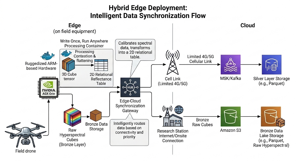
Edge Deployment: Processing at the Source

The bandwidth at some of these remote locations makes a cloud-only approach unrealistic. A 4 GB cube over a 50 Mbps rural LTE connection takes over 10 minutes under ideal conditions, and rural LTE rarely delivers ideal conditions. Multiply that by dozens of passes per day during peak season, and the uplink becomes the dominant bottleneck in the entire system. The first round of processing has to happen on the equipment itself.

One Container, Two Targets

For managing the single OCI-compliant processing container at the edge, both AWS IoT Greengrass and K3s were considered. While Greengrass provides tight, convenience-focused AWS integration for features like device shadows, OTA updates, and managed MQTT bridging, the long-term architectural goal heavily prioritizes operational independence and portability. K3s was the pick here — it runs fully offline after bootstrap, uses standard Kubernetes manifests, and avoids locking the edge layer into a single vendor. This commitment to a lightweight, standard Kubernetes runtime avoids vendor lock-in at the crucial edge layer and provides the essential flexibility needed should a multi-cloud strategy become necessary.

The edge container performs radiometric calibration and spectral flattening, producing a Parquet file that is typically 50–100x smaller than the raw cube. That compression ratio is what makes the entire edge strategy viable — the processed output is small enough to upload over cellular, while the raw cube would take orders of magnitude longer.

Hardware and Sync

Hyperspectral processing is dominated by dense matrix multiplications across hundreds of bands, which requires GPU hardware. The setup uses ruggedized NVIDIA Jetson AGX Orin modules mounted directly on field equipment, providing the CUDA cores needed to run CuPy-based calibration and flattening in near real-time. 

The sync strategy splits on payload size and urgency. Processed Parquet files stream back to the cloud in near real-time via Amazon MSK (Kafka) over an MQTT bridge, giving the lakehouse immediate telemetry. Kafka was chosen over SQS for this link because the downstream Spark Structured Streaming jobs benefit from offset-based replay semantics — if a job fails mid-batch, it resumes from the last committed offset without data loss or duplication, which is harder to guarantee cleanly with SQS visibility timeouts. The raw cubes stay on local storage and are only backhauled when the equipment returns to a facility with a high-speed connection, keeping bandwidth costs under control.

Summary

The core ideas behind this pipeline are straightforward: decouple storage from compute using SQS as a buffer, push the first round of processing to the edge so bandwidth stops being the bottleneck, tier storage aggressively so petabyte-scale retention stays economical, and structure everything into a medallion lakehouse so end users get SQL tables instead of binary blobs. Each piece is well-understood on its own; the value is in how they compose into an end-to-end system that stays reliable and cost-effective at scale.

As noted at the outset, none of this is specific to agriculture. The hyperspectral cube is just one instance of a pattern that shows up across industries — genomics, satellite imagery, LiDAR, manufacturing inspection — wherever heavy payloads are born at the edge and need to become queryable data in the cloud. The crop science forced this architecture into existence, but the blueprint is portable. Swap the payload and the domain-specific transforms, and the rest of the system carries over.