A Developer's Practical Guide to Support Vector Machines (SVM) in Python

Support vector machines (SVMs) are one of the most powerful and versatile supervised machine learning algorithms. Initially famous for their high-performance "out of the box," they are capable of performing both linear and non-linear classification, regression, and outlier detection.

For classification tasks, the core idea behind SVM is to find the optimal hyperplane that best separates the different classes in the feature space.

In this developer's guide, we'll go beyond a simple fit and predict. We'll walk through the essential practical steps to build, tune, and evaluate a high-performance SVM classifier using Python's Scikit-learn library. We will focus on the details that make the difference between a mediocre model and a production-ready one, including data preprocessing, hyperparameter tuning, and a deep dive into evaluation.

This guide will cover:

• How SVMs work (hyperplanes, margins, and the kernel trick).
• A critical, must-do step: Preparing and scaling your data.
• Building a robust training Pipeline.
• Tuning the key hyperparameters (C and gamma) with GridSearchCV.
• Evaluating the model using a confusion matrix and the ROC-AUC score with code and visualizations.

How Do SVMs Work? The Core Concepts

The Linear Case: Hyperplanes and Margins

Imagine you have data points belonging to two different classes on a scatter plot. The goal of an SVM is to draw a line (or a hyperplane in higher dimensions) that separates these two classes.

But it doesn't just draw any line; it finds the optimal line. This optimal hyperplane is the one that has the maximum margin, meaning the largest possible distance between the hyperplane and the nearest data points of each class.

These nearest points, the ones that touch the edge of the margin, are called the "support vectors." They are the most critical data points because they alone define the position and orientation of the decision boundary. This focus on the maximum margin and support vectors is what makes SVMs so robust and effective, as it leads to better generalization on unseen data.

The Non-Linear Case: The Kernel Trick

The real power of SVMs becomes apparent when your data isn't linearly separable. What if your classes are arranged in concentric circles? You can't draw a single straight line to separate them.

This is where the kernel trick comes in. A kernel is a function that takes your low-dimensional data and projects it into a higher-dimensional space where it does become linearly separable.

Imagine your concentric circles in 2D. A kernel function could project this data into 3D, turning the circles into two parallel "bowls," one nested inside the other. Now, in this 3D space, you can easily slide a 2D plane (a hyperplane) right between them to separate the two classes.

The most popular kernel is the Radial Basis Function (RBF) kernel, which is the default in Scikit-learn. It's incredibly flexible and can create complex, non-linear decision boundaries.

Step 1: Preparing Data for SVM (A Critical Step)

This is the most common pitfall for developers new to SVMs. SVMs are not scale-invariant. They work by finding the hyperplane that maximizes the distance of the margins. If one feature (e.g., "Salary" in dollars) ranges from 0 to 1,000,000, while another feature (e.g., "Years of Experience") ranges from 0 to 50, the "Salary" feature will completely dominate the distance calculations. Your model will perform terribly.

Rule #1 of SVMs: You must scale your features before training. The most common method is Standardization (or Z-score normalization), which rescales the data to have a mean of 0 and a standard deviation of 1.

Let's create some sample data to work with.

import numpy as np
import matplotlib.pyplot as plt
import seaborn as sns
from sklearn.datasets import make_classification
from sklearn.model_selection import train_test_split, GridSearchCV
from sklearn.preprocessing import StandardScaler
from sklearn.svm import SVC
from sklearn.pipeline import Pipeline
from sklearn.metrics import (
  classification_report,
  confusion_matrix,
  roc_curve,
  auc,
  RocCurveDisplay
)

# 1. Create a synthetic dataset
# We'll make it non-linear to show the power of the RBF kernel
X, y = make_classification(
  n_samples=1000,
  n_features=2,
  n_informative=2,
  n_redundant=0,
  n_clusters_per_class=1,
  class_sep=0.8, # Make them a bit hard to separate
  random_state=42
) 
# 2. Split into training and testing sets
X_train, X_test, y_train, y_test = train_test_split(X, y, test_size=0.3, random_state=42) 
# 3. Visualize the unscaled data
# We'll plot the test set to see what we're trying to predict
sns.scatterplot(
  x=X_test[:, 0],
  y=X_test[:, 1],
  hue=y_test,
  palette=['#FF5733', '#335BFF'],
  alpha=0.8
) 
plt.title("Unscaled Test Data")
plt.xlabel("Feature 1")
plt.ylabel("Feature 2")
plt.legend(["Class 0", "Class 1"])
plt.show()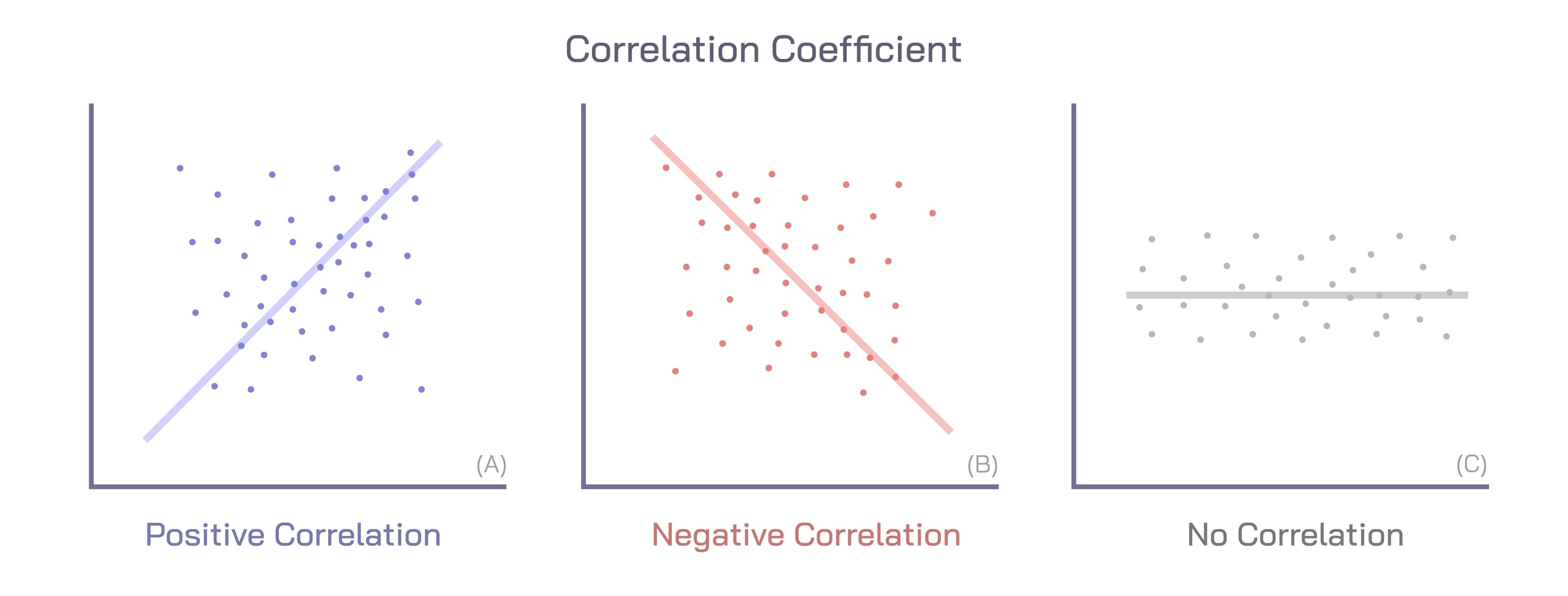

Step 2: Building a Preprocessing and Training Pipeline

Instead of scaling our data manually (scaler.fit_transform(X_train), scaler.transform(X_test)), the best practice is to use a Pipeline.

A Pipeline chains steps together. It will only fit the StandardScaler on the training data and then safely transform both the training and test data. This prevents the cardinal sin of data leakage (letting information from the test set "leak" into your training process).

# Create a pipeline that first scales the data, then trains the SVM
# This is the standard, robust way to do it.

# probability=True is needed later for the ROC-AUC curve
# C and gamma are hyperparameters we will tune
svm_pipeline = Pipeline([
    ('scaler', StandardScaler()),
    ('svm', SVC(kernel='rbf', C=1.0, gamma='auto', probability=True, random_state=42))
 ]) 
# Now, just fit the entire pipeline. It handles scaling automatically.
print("Training the SVM pipeline...")
svm_pipeline.fit(X_train, y_train)
print("Training complete.") 
# Make predictions on the test data
y_pred = svm_pipeline.predict(X_test)

Step 3: Tuning Key Hyperparameters (C and Gamma)

Our pipeline works, but how do we know C=1.0 and gamma='auto' are the best choices? We don't. We need to tune them.

• C (Regularization Parameter): This parameter controls the trade-off between achieving a "clean" (low misclassification) margin and a "wide" (smooth) margin.
  • Low C: A very soft margin. The model allows for more misclassifications in the training data to get a wider, simpler margin. This can prevent overfitting (high bias, low variance).
  • High C: A hard margin. The model tries to classify every training sample correctly. This can lead to a very complex, narrow margin that overfits the training data (low bias, high variance).
• gamma (Kernel Coefficient for 'rbf'): This parameter defines how far the influence of a single training example (a support vector) reaches.
  • Low gamma: A large radius of influence. The model is simpler and smoother. This can lead to underfitting.
  • High gamma: A small radius of influence. Each support vector has a very local "bubble" of influence. This can create highly complex, "island-like" decision boundaries that overfit the data.

We can find the best combination of C and gamma using GridSearchCV (Grid Search Cross-Validation).

# Define the "grid" of parameters to search
# We'll try a few values for C and gamma
param_grid = {
  'svm__C': [0.1, 1, 10, 100],  # Note the 'svm__' prefix
  'svm__gamma': [1, 0.1, 0.01, 0.001]
}

# IMPORTANT: We pass the *pipeline* to GridSearchCV, not just the model.
# This ensures that scaling is part of the cross-validation for each grid combination.
# cv=5 means 5-fold cross-validation. n_jobs=-1 uses all CPU cores.
grid_search = GridSearchCV(
  svm_pipeline,
  param_grid,
  cv=5,
  scoring='roc_auc',
  verbose=2,
  n_jobs=-1
) 
print("Running GridSearchCV to find best C and gamma...") grid_search.fit(X_train, y_train) 
# Get the best model found by the grid search
best_svm = grid_search.best_estimator_ 
print(f"\nBest parameters found: {grid_search.best_params_}") print(f"Best cross-validation ROC-AUC score: {grid_search.best_score_:.4f}") 
# Make new predictions using the *best* model
y_pred_tuned = best_svm.predict(X_test)

Step 4: Evaluating Your Tuned SVM Model

Now that we have tuned our model, let's see how it actually performs on the held-out test data.

The Confusion Matrix: A Deeper Look

The confusion matrix is the foundation for most classification metrics. It gives you a detailed breakdown of your model's predictions versus the actual labels.

• True Positive (TP): Actual was 1, Model predicted 1.
• True Negative (TN): Actual was 0, Model predicted 0.
• False Positive (FP): Actual was 0, Model predicted 1. (Type I Error)
• False Negative (FN): Actual was 1, Model predicted 0. (Type II Error)

From this, Scikit-learn's classification_report calculates:

• Precision: Of all the times the model predicted "Positive," how often was it right? TP / (TP + FP)
• Recall (Sensitivity): Of all the actual "Positive" cases, how many did the model find? TP / (TP + FN)
• F1-Score: The harmonic mean of Precision and Recall. A great all-around metric.

# 1. Classification Report
print("\n--- Classification Report (Tuned Model) ---")
print(classification_report(y_test, y_pred_tuned)) 

# 2. Confusion Matrix
print("\n--- Confusion Matrix (Tuned Model) ---")
cm = confusion_matrix(y_test, y_pred_tuned) 
print(cm) 

# 3. Visualize the Confusion Matrix
plt.figure(figsize=(7, 5))
sns.heatmap(cm, annot=True, fmt='d', cmap='Blues',
            xticklabels=['Predicted 0', 'Predicted 1'],
            yticklabels=['Actual 0', 'Actual 1'])
plt.title('Tuned SVM Confusion Matrix')
plt.ylabel('Actual')
plt.xlabel('Predicted')
plt.show()

The ROC Curve and AUC Score

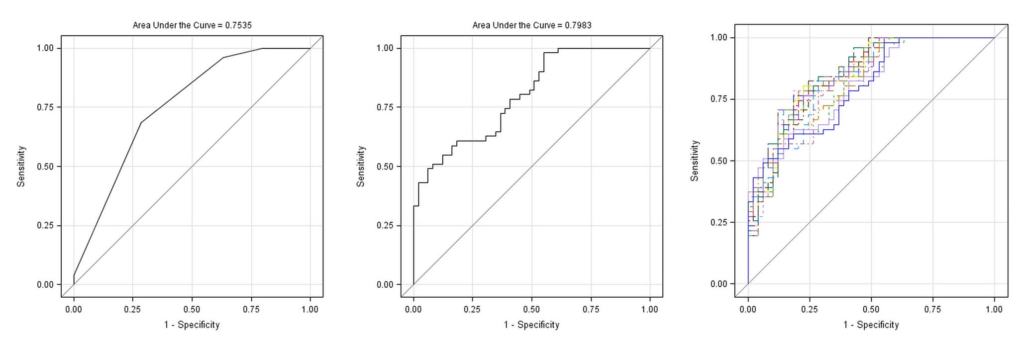
The Receiver Operating Characteristic (ROC) curve is one of the most important evaluation metrics for a binary classifier. It plots the True Positive Rate (Recall) against the False Positive Rate as you vary the decision threshold of the classifier.

The goal is to have a curve that bows as far as possible to the top-left corner.

• Top-Left Corner: A perfect classifier (100% True Positives, 0% False Positives).
• Diagonal Line: A model that is no better than random guessing.

The Area Under the Curve (AUC) summarizes the ROC curve into a single number.

• AUC = 1.0: A perfect classifier.
• AUC = 0.5: A classifier that is no better than random chance.

# We need the predicted *probabilities* for the ROC curve
# This is why we set probability=True in the SVC
y_pred_proba = best_svm.predict_proba(X_test)[:, 1] # Get probabilities for class 1

# Calculate ROC curve
fpr, tpr, thresholds = roc_curve(y_test, y_pred_proba)

# Calculate AUC
roc_auc = auc(fpr, tpr)

print(f"\nTest Set ROC-AUC Score (Tuned Model): {roc_auc:.4f}")

# Plot the ROC curve
plt.figure(figsize=(8, 6))
plt.plot(fpr, tpr, color='blue', lw=2, label=f'Tuned SVM (AUC = {roc_auc:.4f})')
plt.plot([0, 1], [0, 1], color='gray', lw=2, linestyle='--', label='Random Chance (AUC = 0.50)')
plt.xlim([0.0, 1.0])
plt.ylim([0.0, 1.05])
plt.xlabel('False Positive Rate')
plt.ylabel('True Positive Rate')
plt.title('Receiver Operating Characteristic (ROC) Curve')
plt.legend(loc="lower right")
plt.grid(True)
plt.show()

An AUC score (e.g., 0.97) indicates a high-performing model that is excellent at distinguishing between the two classes.

Conclusion

The Support Vector Machine is a robust and effective algorithm, but only when used correctly. We've seen that SVMs are not a simple "plug-and-play" model.

By following this guide, you've moved from a basic concept to a production-ready approach. You now know that feature scaling is mandatory, not optional. You know how to use a Pipeline to prevent data leakage and streamline your workflow. And, most importantly, you know how to tune the critical C and gamma hyperparameters to build a model that truly generalizes, and then prove its performance with a confusion matrix and ROC-AUC curve.