Predicting Stock Data With Cassandra and TensorFlow

The scenario that this blog will cover is a time-series forecasting of a specific stock price. The problem itself is very common and widely known. That being said, this is a technology demo and is in no way intended as market advice. The purpose of the demo is to show how Astra and TensorFlow can work together to do time-series forecasting. The first set is setting up your database.

Getting Test Data

Now that you have the database, credentials, and bundle file on your machine, let’s ensure you get the data needed to run this tutorial. This data is open source and available on many platforms. One of which is the Kaggle platform, where people have already done the work of gathering this data via APIs. 

Here is the link to that data. 

Another source that can fit into this problem is the Tesla dataset, which is also open on GitHub. 

The simplest option, which we recommend as well, is to clone our Github repository (which we will cover anyway), where we also added sample data for you to jump right into the code.

Now, let’s jump right into the code!

Code for the Tutorial

The code for this tutorial can be found under our repo link on GitHub. If you are already familiar with Git and JupyterLabs just go ahead and clone and rerun the notebook steps using Git clone.

The readme on the repo should also have all the details needed to get started with that code. 

Using the Repo 

In this section, we make sure to cover some of the steps you’ll need to follow to complete the tutorial and highlight some of the needed details.

After cloning the code, navigate to the project directory and start by installing the dependencies (note that if you are using the GitPod deployment method, then this will happen automatically) using the following command:

pip install -r requirements.txt

Note that the Python version used in this example is 3.10.11, so make sure you either have that installed or make sure create a virtual environment using pyenv (whatever works best for you).

Jupyter[Lab] Installation

Last but not least, before jumping to running the code, make sure you have Jupyter installed on your machine. You can do that by running the command below.

pip install jupyterlab

Note that here we are installing JupyterLab, which is a more advanced version of Jupyter notebooks. It offers many features in addition to the traditional notebooks.

Once installed, type jupyter-lab in the terminal. It should open a window in your browser listing your working directory’s content. If you are in the cloned directory, you should see the notebook and should be able to follow the steps. 

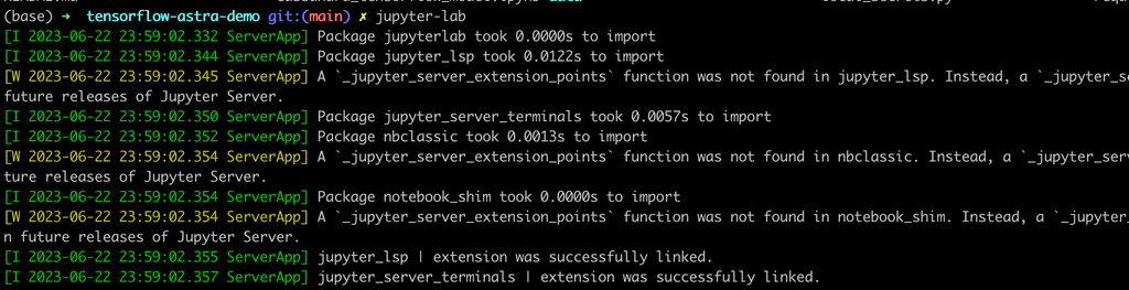
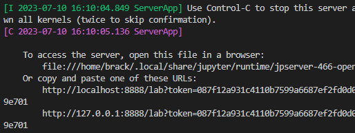
If it doesn’t start automatically, you can navigate to the JupyterLabs server by clicking on the URLs in your terminal:

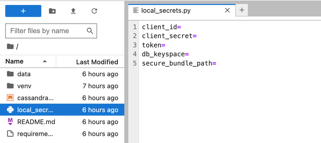
Now that you’ve run the Jupyter command from your working directory, you should see the project tree in your browser and navigate to the files. First, let’s make sure we configure the secrets before starting any coding, so make sure you open the local_secrets.py file and fill in the details provided/extracted from the AstraDB website after setting up the database details.

Now, we can navigate to the notebook. Let’s start by reading the data and storing it in AstraDB.

Storing the Data in AstraDB

This step is doing nothing but showcasing the fact that you can use AstraDB to feed data to your models. AstraDB is, above all else, a powerful and scalable database. Data has to be stored somewhere, and whether you are on Astra or Cassandra already or just getting started with the tools, this tutorial shows you how easy it is to use Astra for your backend.

It’s easy to use the CQL language to create a table and load the sample data from this tutorial into it. The logic should be as follows:

# Create training data table

query = """

CREATE TABLE IF NOT EXISTS training_data (

    date text,

    open float,

    high float,

    low float,

    close float,

    adj_close float,

    volume float,

    PRIMARY KEY (date)

)

"""

session.execute(query)



# Load the data into your table



for row in data.itertuples(index=False):

    query = f"INSERT INTO training_data (date, open, high, low, close, adj_close, volume) VALUES ('{row[0]}', {row[1]}, {row[2]}, {row[3]}, {row[4]}, {row[5]}, {row[6]})"

    session.execute(query)

Once done with the previous step, let’s read the data again and make sure we order it as a time series forecasting problem. This is a data management step to make sure data is ordered for the series.

Use the code below to read the data for your time series and prepare it for use by TensorFlow:

# Retrieve data from the table

query = "SELECT * FROM training_data"

result_set = session.execute(query)

# Convert the result set to a pandas DataFrame:

data = pd.DataFrame(list(result_set)).sort_values(by=['date'])

Analyzing the Data

We can now write some code to understand and analyze the data with some graphics. The below chart, for example, shows the Open and Close prices of the stock (the price when the market opens and when the market closes) for the timeframe of 4 years between 2016 and 2020.

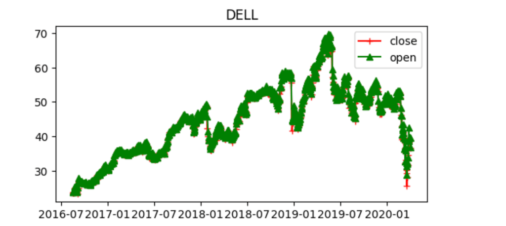
You can find more graphs in the notebook describing some other factors and analyzing the fluctuation of the prices over time.

Let’s move now to building the model itself.

Building the Model

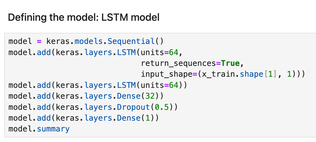
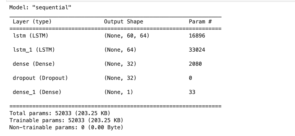
For this example, we will be using an LSTM model (or Long Short Term Model), a deep learning model known for its capability to recognize patterns in the data, which works well with the problem we are demonstrating.

It’s also important to note that we will use Keras (a deep learning API for Python) as a backend for our TensorFlow example. The model is composed of 2 LSTM layers: one dense layer, one dropout layer, and finally, another dense layer. 

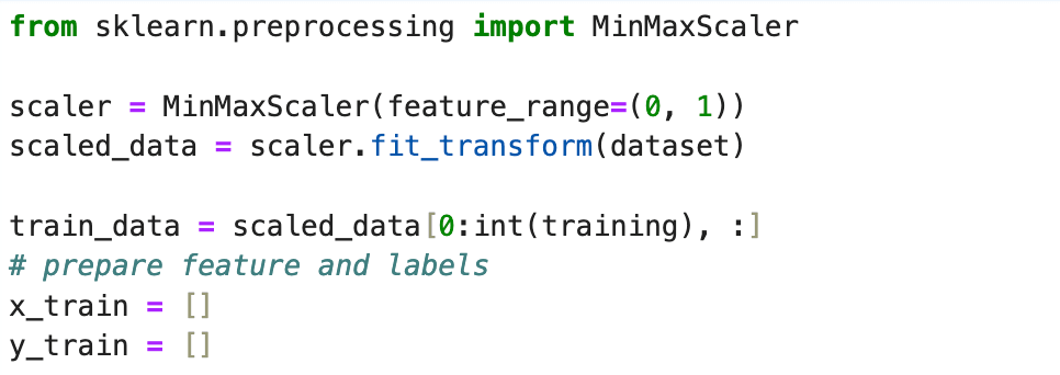
Another important aspect to note is the data normalization and scaling.

The model’s performance is very sensitive to the scale and variation of the actual data values; thus, it’s crucial to normalize the data and transform it into a consistent range or distribution. We’ve used one of the most popular scalers in machine learning, the min-max scaler for data normalization. We also implemented the data splitting into train and test sets. 

In this case, and for the sake of the demo, we used 95% of the data as training, and the rest is for testing.

Once done transforming and configuring the data and the model, we can start the fit step also known as the training step. 

Using the Data

Once you have the model trained on the training data, you’ll be able to use it to make a time series prediction. 

Running the following command will generate the predicted data:

predictions = model.predict(x_test)

But note that since we’ve scaled our values using our minMaxScaler, the generated predictions at this point are all within the scaling range, and to get them back to the original scale, we will need to inverse what we’ve done with Tensorflow; doing that is as simple as running the following line of code.

predictions = scaler.inverse_transform(predictions)

The following graph shows the training data evolution over time as well as the test vs. forecast generated by our model.

Notice the different colors at the far right of the graph. The orange color is the testing subset of the actual data. The green line represents the forecasted stock price. In this case, our forecasting did a relatively good job predicting the drop in stock price. That Predictions line is the main outcome of any forecast. 

Note that for this regression problem, we’ve also used some model evaluation metrics. MSE and RMSE were used for that matter, and below is the snippet of code corresponding to their implementation:

# evaluation metrics

mse = np.mean(((predictions - y_test) ** 2))

rmse = np.sqrt(mse)

Model Storage

Let’s now move on to model storage. In this section, we will interact again with our database AstraDB and, more specifically, storing the model and the error metrics in a table. We picked a simple structure for this for visibility purposes. 

The table schema is as follows: 

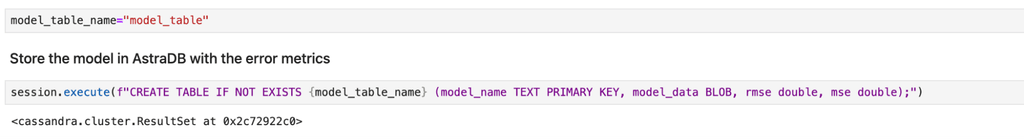
The model data itself will be stored as a blob; for this, we will need to take our model data, convert it into JSON, and then store it in our table. The below code describes how you can do this easily:

Now that we’ve stored our model’s data, we can write some logic to retrieve it again for different purposes. We can load the model, serve it, and run some forecasting on the fly, or we can also reload it and run the model on some batched data to run some batch forecasting.

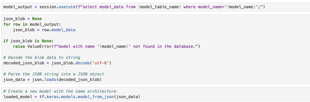
Reading the Model

Here is the code that allows reading the model. Based on the need, you can run any of the forecasting approaches. 

We can also take a look at the model’s summary and make sure that it corresponds exactly to what we trained and stored previously: 

loaded_model.summary()

You should see something like this: 

And you’ve made it to the end of this tutorial!

As we wrap up this blog, you’ve now learned how to interact with AstraDB and use it as a source of your model’s artifacts and data. 

Conclusion

In this blog, we explored the powerful combination of TensorFlow and AstraDB. Throughout the tutorial, we covered essential steps, such as setting up the environment, installing the necessary dependencies, and integrating TensorFlow with AstraDB. We explored how to perform common tasks like data ingestion, preprocessing, and model training using TensorFlow's extensive library of functions. Additionally, we discussed how AstraDB's flexible schema design and powerful query capabilities enable efficient data retrieval and manipulation.

By combining TensorFlow and AstraDB, developers can unlock a world of possibilities for creating advanced machine-learning applications. From large-scale data analysis to real-time predictions, this powerful duo empowers us to build intelligent systems that can handle massive datasets and deliver accurate results.