Reinforcement Learning Overview
And no, we're not talking about Pavlov's dogs here. Learn about the reinforcement learning aspect of machine learning and the key algorithms that are involved!
Join the DZone community and get the full member experience.
Join For FreeThere are basically three different types of machine learning:
- Supervised learning: The major use case is prediction. We provide a set of training data including the input and output, then train a model that can predict the output from an unseen input.
- Unsupervised learning: The major use case is pattern extraction. When we provide a set of data that has no output, the algorithm will try to extract the underlying non-trivial structure within the data.
- Reinforcement learning: The major use case is optimization. Mimicking how humans learn from childhood, we use a trial-and-error approach to find out what actions will produce good outcomes and bias our preference towards those good actions.
In this post, I will provide an overview of the settings of reinforcement learning as well as some of its key algorithms.
Agent/Environment Interaction
Reinforcement learning is all about how we can make good decisions through trial and error. It is the interaction between the "agent" and the "environment."
Repeat the following steps until you reach a termination condition:
- The agent observes the environment having state s.
- Out of all possible actions, the agent needs to decide which action to take. This is called "policy," which is a function that outputs an action given the current state.
- The agent takes the action and the environment receives that action.
- Through a transition matrix model, the environment determines the next state and proceeds to that state.
- Through a reward distribution model, the environment determines the reward to the agent given he take action a at state s.

The agent's goal is to determine an optimal policy such that the value of the start state is maximized.
- Episode: A sequence of (s1, a1, r1, s2, a2, r2, s3, a3, r3 ... st, at, rt ... sT, aT, rT).
- Reward rt: Money the agent receives after taking action at a state at time t.
- Return: Cumulative reward since the action is taken (sum of rt, r[t+1], ... rT).
- Value: Expected return at a particular state, called state value or V(s), or the expected return when taking action a at state s, called Q value or Q(s,a).
The optimal policy can be formulated as choosing action a* and the amount of all choices of a at state s such that Q(s, a*) is the maximum.
To deal with these never-ending interactions, we put a discount factor "gamma" on future rewards. This discount factor will turn the sum of an infinite series into a finite number.
Optimal Policy When Model Is Known
If we know the model, then figuring out the policy is easy. We just need to use dynamic programming techniques to compute the optimal policy offline so that there's no need for learning.
Two algorithms can be used.
Value Iteration
Value iteration starts with a random value, iteratively updates the value based on Bellman's equation, and finally, computes the value of each state or state/action pair (also called Q state). The optimal policy for a given state s is to choose the action a* to maximize the Q value, Q(s, a).

Policy Iteration
Policy iteration starts with a random policy and iteratively modifies the policy to make it better until the policy at the next iteration doesn't change anymore.

However, in practice, we usually don't know the model, so we cannot compute the optimal policy as described above.
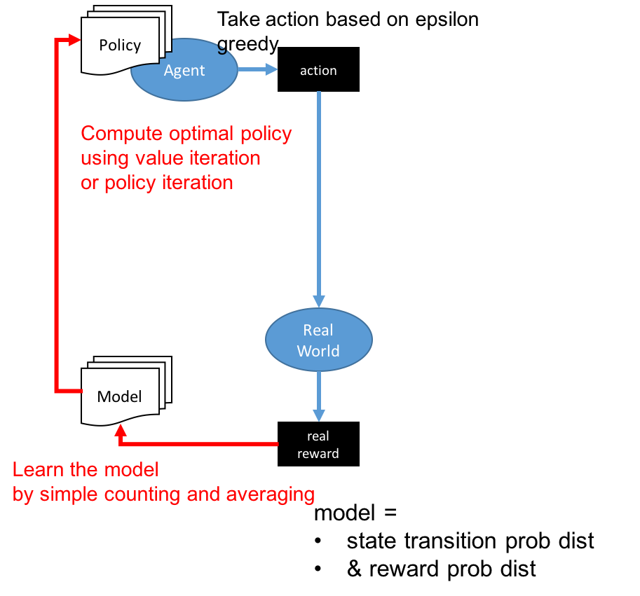
Optimal Policy When Model Is Unknown
One solution is model-based learning. We spare some time to discover the transition probability model and the reward distribution model. To make sure we experience all possible combinations of different state/action pairs, we will take random actions in order to learn the model.
Once we learn the model, we can go back to use the value iteration or policy iteration to determine the optimal policy.
Learning has a cost, though. Rather than taking the best action, we will take random actions in order to explore new actions that we haven't tried before. It's very likely that the associated reward is not the maximum. However, we accumulate our knowledge about how the environment reacts under a wider range of scenarios to get a better action in the future. In other words, we sacrifice or trade-off in the short term gain for a long-term gain.
Having the right balance is important. A common approach is to use the epsilon greedy algorithm. For each decision step, we allocate a small probability e where we take a random action and probability (1-e) where we take the best-known action that we've already explored.
Another solution approach is model-free learning. Let's go back to look at the detailed formula under value iteration and policy iteration so that we can better calculate the expected value of state value and Q value. Can we figure out the expected state and Q value through trial and error?
Value-Based, Model-Free Learning
If we modify the Q value iteration algorithm to replace the expected reward/next state with the actual reward/next state, we arrive at the SARSA algorithm below.

Deep Q Learning
The algorithm above requires us to keep a table to remember all Q(s,a) values — which can be huge and also may become infinite if any of the states or actions are continuous. To deal with this, we will introduce the idea of the value function. The state and action will become the input parameters of this function, which will create input features, feed into a linear model, and finally output the Q value.

- Instead of looking up the Q(s,a) value, we call the function (which can be a DNN) to pass in the f(s, a) feature and get its output.
- We randomly initialize the parameter of the function (which can be weighted if the function is a DNN).
- We update the parameters using gradient descent on the list, which can be the difference between the estimated value and the target value (it can be a one-step look-ahead estimation: r + gamma*max_a'[Q(s',a)]).

If we further generalize the Q value function using a deep neural network, update the parameter using back propagation, and reach a simple version of deep Q learning.
Policy Gradient
- If the action is discrete, it outputs a probability distribution of each action.
- If the action is continuous, it outputs the mean and variance of the action, assuming normal distribution.
The agent will sample from the output distribution to determine the action, so
itschosen action is stochastic (non-deterministic). Then, the environment will determine the reward and next state. And the cycle repeats. The goal is to find the best policy function where the expected value of Q(s, a) is maximized. Notice that s and a are random variables parameterized by θ.

To maximize an expected value of a function with parameters θ, we need to calculate the gradient of that function.

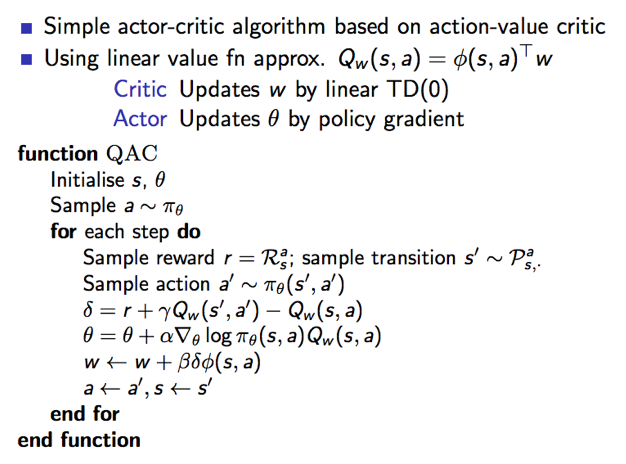
Actor Critic Algorithm
There are two important notes about this equation:
- To improve the policy function, we need an accurate estimation of Q value and also need to know the gradient of log(s, a).
- To make the Q value estimation more accurate, we need a stable policy function.
We can break down these into two different roles:
- An actor whose job is to improve the policy function by tuning the policy function parameters.
- A critic whose job is to fine tune the estimation of Q value based on current (incrementally improving) policy.
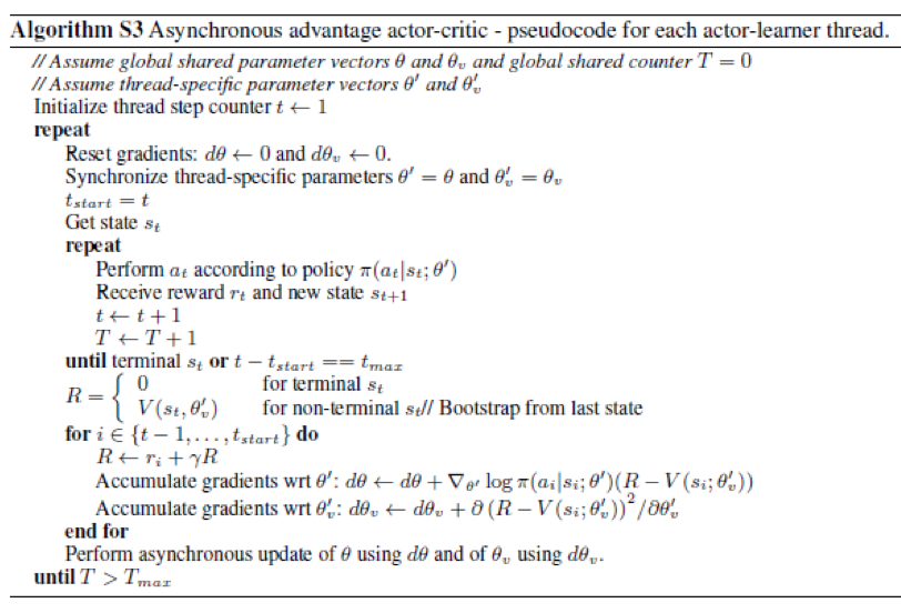
Then we enhance this algorithm by adding the following steps:
- Replace the Q value function with an Advantage function, where A(s, a) = Q(s, a) - expected Q(s, *), i.e. A(s, a) = Q(s, a) - V(s).
- Run multiple threads asynchronously.
This is a state-of-the-art A3C algorithm:
References
Published at DZone with permission of Ricky Ho. See the original article here.
Opinions expressed by DZone contributors are their own.
Comments