When Coalesce Is Slower Than Repartition: A Spark Performance Paradox

If you've worked with Apache Spark, you've probably heard the conventional wisdom: "Use coalesce() instead of repartition() when reducing partitions — it's faster because it avoids a shuffle." This advice appears in documentation, blog posts, and is repeated across Stack Overflow threads. But what if I told you this isn't always true?

In a recent production workload, I discovered that using repartition() instead of coalesce() resulted in a 33% performance improvement (16 minutes vs. 23 minutes) when writing data to fewer partitions. This counterintuitive result reveals an important lesson about Spark's Catalyst optimizer that every Spark developer should understand.

The Conventional Wisdom

Let's quickly recap the standard guidance:

• coalesce(n): Reduces the number of partitions without a full shuffle. It combines existing partitions, making it a narrow transformation. Best for reducing partitions after filtering operations.
• repartition(n): Performs a full shuffle to redistribute data evenly across partitions. It's a wide transformation involving network I/O. Can increase or decrease partition count.

The general rule? Use coalesce() for reducing partitions to avoid expensive shuffle operations.

The Problem: Small Files Syndrome

In my scenario, I needed to write output data to 40 files, but my shuffle partition count was set to 1280 (default parallelism). Without intervention, this would create 1,280 small files of approximately 20 MB each — a classic small files problem that plagues data lakes and degrades query performance.

The solution seemed obvious: use coalesce(40) before writing. But the execution time was disappointing: 23 minutes.

Out of curiosity, I tried repartition(40) instead. The result? 16 minutes — a 30% improvement despite adding a shuffle operation!

The Hidden Culprit: Catalyst Optimizer's Pushdown

Here's what's happening under the hood, and why it catches developers off guard:

Coalesce Gets Pushed Down

Spark's Catalyst optimizer is smart — sometimes too smart. When you write code like this:

df.load()
  .map(...)
  .filter(...)
  .join(...)
  .coalesce(10)
  .save()

You expect coalesce() to execute just before the write operation. However, Catalyst pushes the coalesce operation as early as possible in the execution plan. Your code effectively becomes:

df.load()
  .coalesce(10)  // Pushed to the beginning!
  .map(...)
  .filter(...)
  .join(...)
  .save()

The Parallelism Bottleneck

This optimization creates a critical bottleneck: your entire job now runs with limited parallelism.

In my case:

• With coalesce(40): A critical stage processed 1,792 MB of data using only 40 tasks across 40 cores, taking 8.8 minutes
• With repartition(40): The same stage used 200 tasks with full cluster parallelism, then added a shuffle stage to redistribute to 40 partitions

The additional shuffle stage in repartition() added overhead, but the massive parallelism gain in earlier stages more than compensated for it.

The Evidence: Stage-by-Stage Breakdown

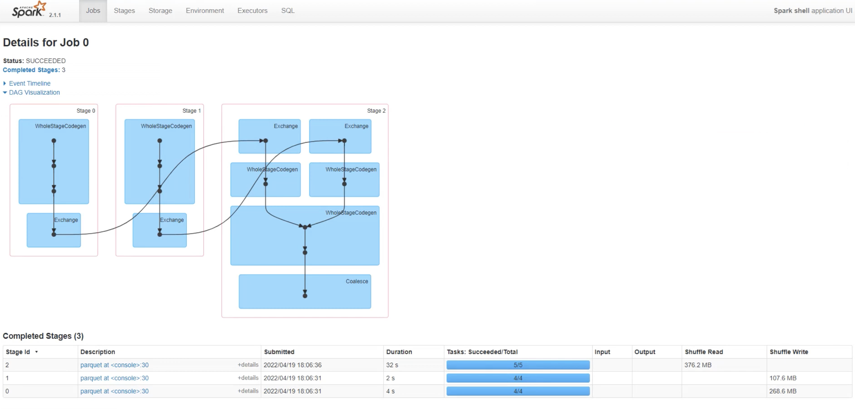
Coalesce Execution (23 Minutes Total)

• Stage 0: 32 seconds | 4 tasks | Shuffle Write: 268.6 MB
• Stage 1: 2 seconds | 4 tasks | Shuffle Read: 376.2 MB | Shuffle Write: 107.6 MB
• Stage 2: 4 seconds | 5 tasks | Output: 107.6 MB
• Total Stages: 3
• Bottleneck: Limited to 40 cores throughout processing

Repartition Execution (16 Minutes Total)

• Stage 3: 4 seconds | 4 tasks | Shuffle Write: 268.6 MB
• Stage 4: 2 seconds | 4 tasks | Shuffle Read: 376.2 MB | Shuffle Write: 231.6 MB
• Stage 5: 8 seconds | 200 tasks | Shuffle Read: 231.6 MB | Shuffle Write: 107.6 MB
• Stage 6: 6 seconds | 5 tasks | Output: 107.6 MB
• Total stages: 4
• Key advantage: 200 tasks with full parallelism in Stage 5

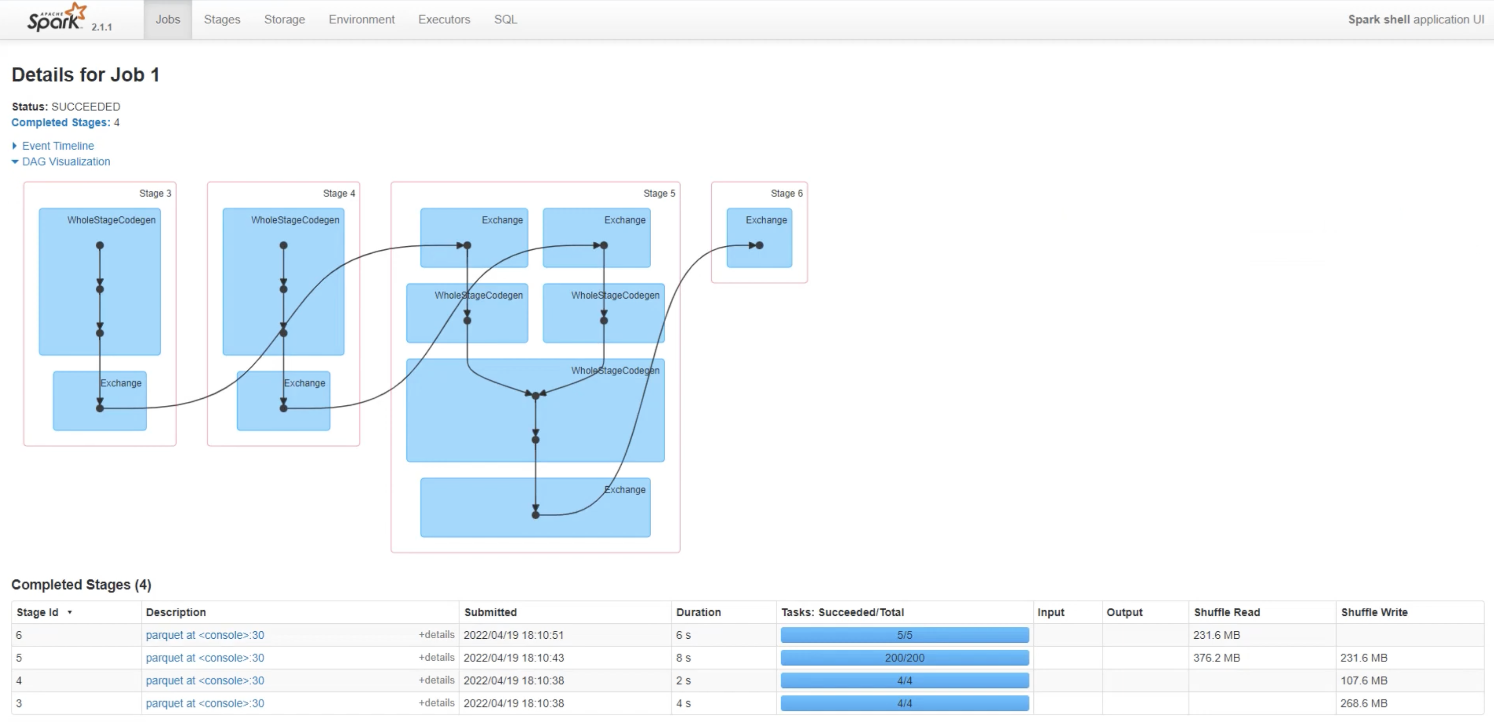
The extra stage in repartition() is offset by the ability to leverage 200 parallel tasks (vs. 40) during data processing.

Here's the simplified reproduction case:

// Coalesce approach
val df1 = spark.range(1, 50000000).toDF("id")
  .withColumn("c1", lit("NA"))
val df2 = spark.range(25555555, 45555555).toDF("id2")
  .withColumn("c2", lit("NA"))
val df3 = df1.join(df2, df1("id") === df2("id2"), "inner")

println("No of partitions: " + df3.rdd.getNumPartitions)
df3.coalesce(5)
  .write.mode("overwrite")
  .parquet("/path/to/coalesce_output")

// Repartition approach
val df4 = spark.range(1, 50000000).toDF("id")
  .withColumn("c1", lit("NA"))
val df5 = spark.range(25555555, 45555555).toDF("id2")
  .withColumn("c2", lit("NA"))
val df6 = df4.join(df5, df4("id") === df5("id2"), "inner")

println("No of partitions: " + df6.rdd.getNumPartitions)
df6.repartition(5)
  .write.mode("overwrite")
  .parquet("/path/to/repartition_output")

When to Use What: Decision Framework

Use coalesce() when:

• Reducing partitions after aggressive filtering (data size significantly reduced)
• The coalesced partition count is still reasonably high (not a drastic reduction)
• You're at the very end of processing with no significant operations remaining
• Data is already relatively balanced across partitions

Use repartition() when:

• Reducing partitions drastically (e.g., 1280 → 40)
• You have significant processing before the write operation
• Data skew is present and needs rebalancing
• You need to increase partition count
• The cost of shuffle is justified by maintaining full parallelism

Key Takeaways

1. Catalyst optimization isn't always optimal: The optimizer makes assumptions that may not fit your use case
2. Parallelism matters more than shuffle avoidance: A shuffle with full parallelism often beats limited parallelism without shuffle
3. Check the execution plan: Use explain() and the Spark UI to understand what's actually happening
4. Context is king: Performance tuning requires understanding your specific data characteristics and cluster resources
5. Test both approaches: When dealing with large partition reductions, benchmark both methods

Conclusion

The coalesce() vs. repartition() decision isn't as straightforward as the documentation suggests. While coalesce() avoids shuffle overhead, it can inadvertently throttle your job's parallelism through optimizer pushdown, especially when drastically reducing partition counts.

The lesson? Always profile your Spark jobs. The Spark UI is your friend — examine stage durations, task counts, and shuffle metrics. What works in theory doesn't always work in production, and sometimes the "expensive" operation (shuffle) enables optimizations that more than pay for themselves

Disclaimer: The opinions expressed in this article are solely those of the author and do not represent the opinions or positions of any organization or employer.