SQL Extensions for Time-Series Data in QuestDB
A short hands-on tutorial on how to use SQL extensions built for time-series data in QuestDB.
Join the DZone community and get the full member experience.
Join For FreeIn this tutorial, you are going to learn about QuestDB SQL extensions which prove to be very useful with time-series data. Using some sample data sets, you will learn how designated timestamps work and how to use extended SQL syntax to write queries on time-series data.
Introduction
Traditionally, SQL has been used for relational databases and data warehouses. However, in recent years there has been an exponential increase in the amount of data that connected systems produce, which has brought about a need for new ways to store and analyze such information. For this reason, time-series analytics have proved critical for making sense of real-time market data in financial services, sensor data from IoT devices, and application metrics.
This explosion in the volume of time-series data led to the development of specialized databases designed to ingest and process time-series data as efficiently as possible. QuestDB achieves this while supporting standard ANSI SQL with native extensions for time series analysis.
Apart from that, QuestDB also makes the syntax easier by implementing implicit clauses. It also includes a random data generation feature which is extremely useful for exploring the functionality of the database as well as in database testing. Although there is much to talk about QuestDB’s SQL dialect, in this tutorial, you will learn about SQL extensions.
Throughout this tutorial, we’ll be using two data sets. The first one is taxi trip data for New York City for the month of February 2018. It contains information about the number of passengers, trip fare, tip amount, and the start date and time of the trip. You can find out the average earnings per number of passengers, the tipping behavior of NYC taxi riders, the busiest times of the day, and so on.
The second data set contains weather information for ten years, starting from 1st January 2010 to 1st January 2020. This dataset contains information about temperature, wind speed, rainfall, depth of snow, visibility, and more. You can use this data to analyze how weather patterns emerge over long periods of time. You can also compare the weather at the same time of the year for different years. To get started, you can install the aforementioned data sets using the following shell script:
docker run -p 8812:8812 -p 9000:9000 questdb/questdb

curl https://s3-eu-west-1.amazonaws.com/questdb.io/datasets/grafana_tutorial_dataset.tar.gz > grafana_data.tar.gz
tar -xvf grafana_data.tar.gz

curl -F data=@taxi_trips_feb_2018.csv http://localhost:9000/imp
curl -F [email protected] http://localhost:9000/imp
SQL Extensions
While implementing ANSI SQL to the greatest extent, QuestDB has introduced some time-series-specific SQL extensions to enhance the performance and query reading and writing experience of the database users and developers. Let’s look into all of the SQL extensions one by one.
Timestamp Search
A time-series database isn’t complete if it doesn’t provide a method to search across time. In QuestDB, you can partition tables by time intervals. Each partition will be saved in a separate set of files on the disk. To provide a relational database-like optimization of pruning partitions, QuestDB offers the feature of Timestamp search.
To benefit from this feature, a table should have a designated timestamp column. Any timestamp column can be marked as the designated timestamp column either while creating the table or while creating temporary sub-tables within a query. The designated timestamp column forces the table to have records in increasing time order. Hence, it implicitly enforces a constraint that rejects any out-of-order inserts. Rather than rejecting the out-of-order inserts, QuestDB is already working on accepting delayed records out of order. Timestamp search can also be performed using the normal ≥, ≤, <, > operators, but it is not as efficient as it is using designated timestamps.
Another benefit of designated timestamp column is that it enables the efficient use of
ASOFjoins which are specialized joins to join tables based on timestamp where timestamps don’t match exactly. A prerequisite for using getting deterministic results from anASOFjoin is that the data in the table should be ordered by time. Designated timestamp columns enforce time ordering in a table.
The two sample data sets were imported directly from a CSV file, and a table was created on-the-fly. Although you can create a designated timestamp while importing the data, it is important to understand how to deal with tables that don’t have a designated timestamp. So, let’s create the designated timestamp now and partition the two tables by month.
SQL script to CTAS imported datasets to create Designated Timestamp columns.
RENAME TABLE taxi_trips_feb_2018.csv TO taxi_trips_unordered;
RENAME TABLE weather.csv to weather_unordered;

CREATE TABLE taxi_trips AS (
  SELECT * FROM taxi_trips_unordered ORDER BY pickupDatetime
) timestamp(pickupDatetime)
PARTITION BY MONTH;

CREATE TABLE weather AS (
  SELECT * FROM weather_unordered ORDER BY timestamp
) timestamp(timestamp)
PARTITION BY MONTH;
Using designated timestamp search notation, you can simplify your timestamp-based searches on tables. The following example queries the weather dataset. In this example, you can see that the same operator can be used to query many different time ranges. The first part UNION will give you the count of records for the whole year of 2019, while the second part UNION will give you the count of records for the month of December 2019, and so on.
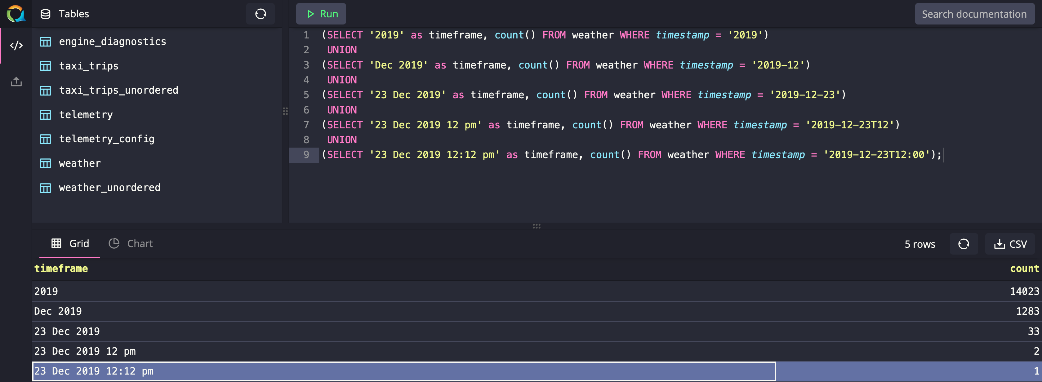
(SELECT '2019' as timeframe, count() FROM weather WHERE timestamp = '2019')
 UNION
(SELECT 'Dec 2019' as timeframe, count() FROM weather WHERE timestamp = '2019-12')
 UNION
(SELECT '23 Dec 2019' as timeframe, count() FROM weather WHERE timestamp = '2019-12-23')
 UNION
(SELECT '23 Dec 2019 12 pm' as timeframe, count() FROM weather WHERE timestamp = '2019-12-23T12')
 UNION
(SELECT '23 Dec 2019 12:12 pm' as timeframe, count() FROM weather WHERE timestamp = '2019-12-23T12:00');
LATEST BY
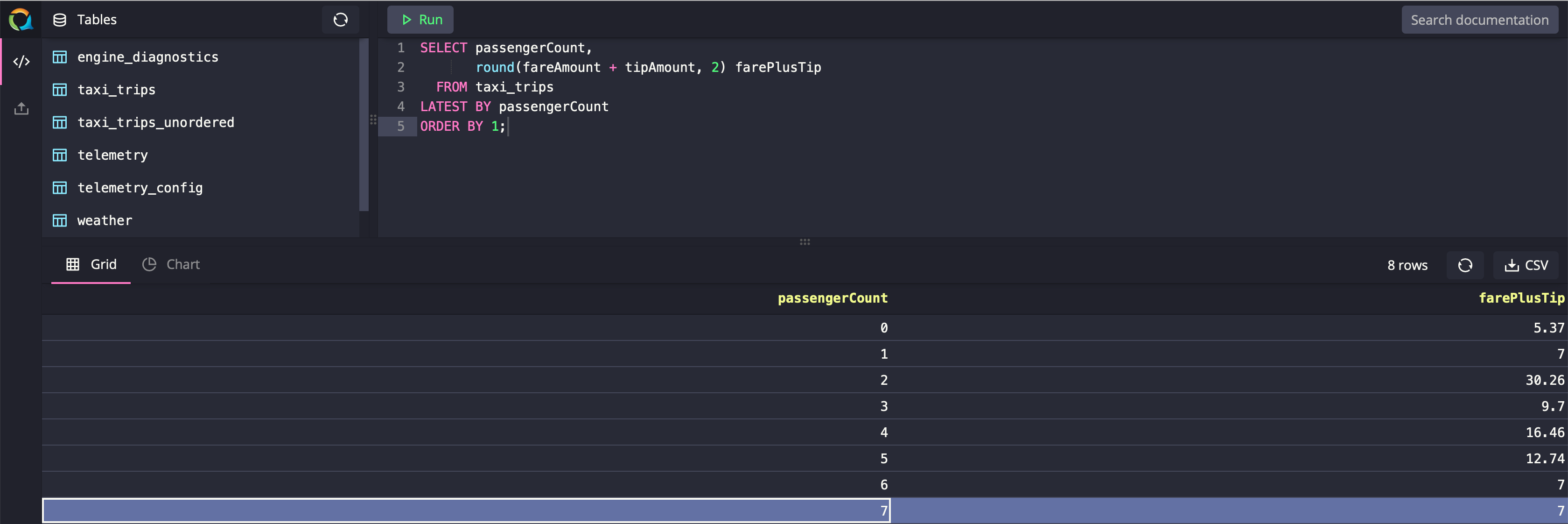
This SQL extension finds the latest entry for a given key or combination of keys by timestamp. The functionality of LATEST BY is similar to functions like FIRST, FIRST_VALUE, etc., which are available in traditional relational databases and data warehouses.
In a relational database, you’d either have to first find out the latest timestamp and, using a subquery, find the farePlusTip amount for the passengerCount, or you’d have to use one of the aforementioned analytic functions like FIRST_VALUE. QuestDB makes life easier for database users and developers by creating a new clause for serving the purpose of finding the latest records per group.
In the following example, you will see that using LATEST BY clause, based on the passengerCount, we can find out what the farePlusTrip was for the latest trip completed.

xxxxxxxxxx
SELECT passengerCount,
round(fareAmount + tipAmount, 2) farePlusTip
FROM taxi_trips
LATEST BY passengerCount
ORDER BY 1;
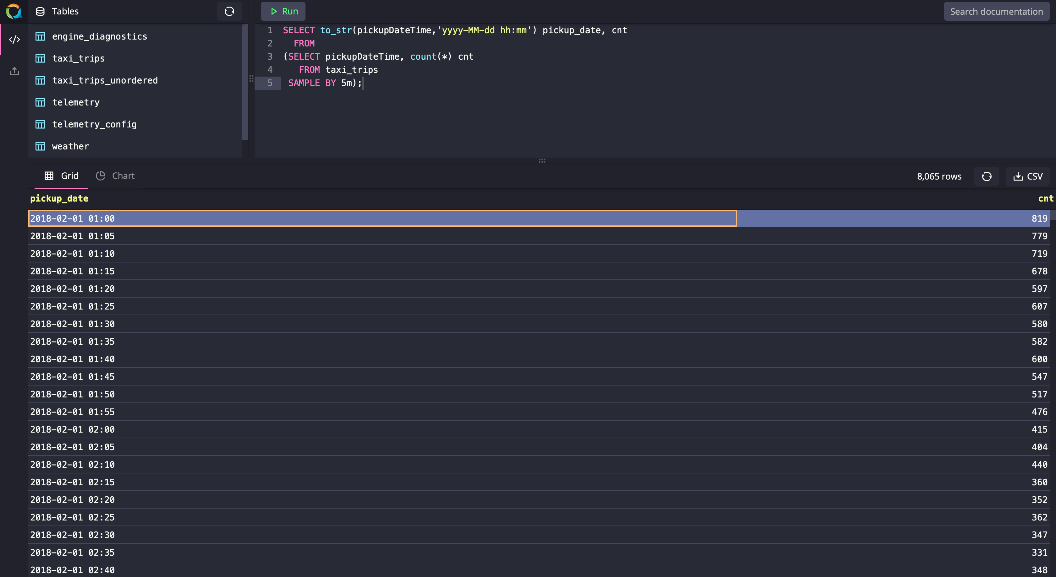
SAMPLE BY
This is another extension that is optimal for time-series data as it allows the grouping of data based on timestamps without explicitly providing timestamp ranges in the where clause. You can bucket your data into chunks of time using this extension.
In regular SQL, you’d need to use a combination of CASE WHEN statements, GROUP BY clauses, and WHERE clauses to get similar results. QuestDB SAMPLE BY does the trick. To use this SQL extension, you need to make sure that the table has a designated timestamp column.
In the following example, you’ll see the data is sampled or grouped by day using 24h the SAMPLE_SIZE in the SAMPLE BY clause. Depending upon the frequency of data ingested into the table, you might need to adjust the size of the bucket by adjusting. SAMPLE_SIZE.
It is common in time-series databases to have really low granularity. Hence, it is common to have data grouped by intervals of time ranging from seconds to years. Here are some more examples demonstrating how to go about using the SAMPLE BY clause for different sample sizes:
SELECT to_str(pickupDateTime,'yyyy-MM-dd hh:mm:ss') pickup_date, cnt
  FROM
(SELECT pickupDateTime, count(*) cnt
   FROM taxi_trips
 SAMPLE BY 20s);

SELECT to_str(pickupDateTime,'yyyy-MM-dd hh:mm') pickup_date, cnt
  FROM
(SELECT pickupDateTime, count(*) cnt
   FROM taxi_trips
 SAMPLE BY 5m);

SELECT to_str(pickupDateTime,'yyyy-MM-dd') pickup_date, cnt
  FROM
(SELECT pickupDateTime, count(*) cnt
   FROM taxi_trips
 SAMPLE BY 24h);

SELECT to_str(pickupDateTime,'yyyy-MM-dd') pickup_date, cnt
  FROM
(SELECT pickupDateTime, count(*) cnt
   FROM taxi_trips
 SAMPLE BY 7d);
Changes to the Usual SQL Syntax
Apart from the SQL extensions, there are a few changes to the usual SQL syntax to enhance the database user experience. The changes are related to GROUP BY and HAVING clauses. The idea behind doing this is to simplify query writing and improve the readability and ease of use of the SQL dialect while Reducing SQL verbosity.
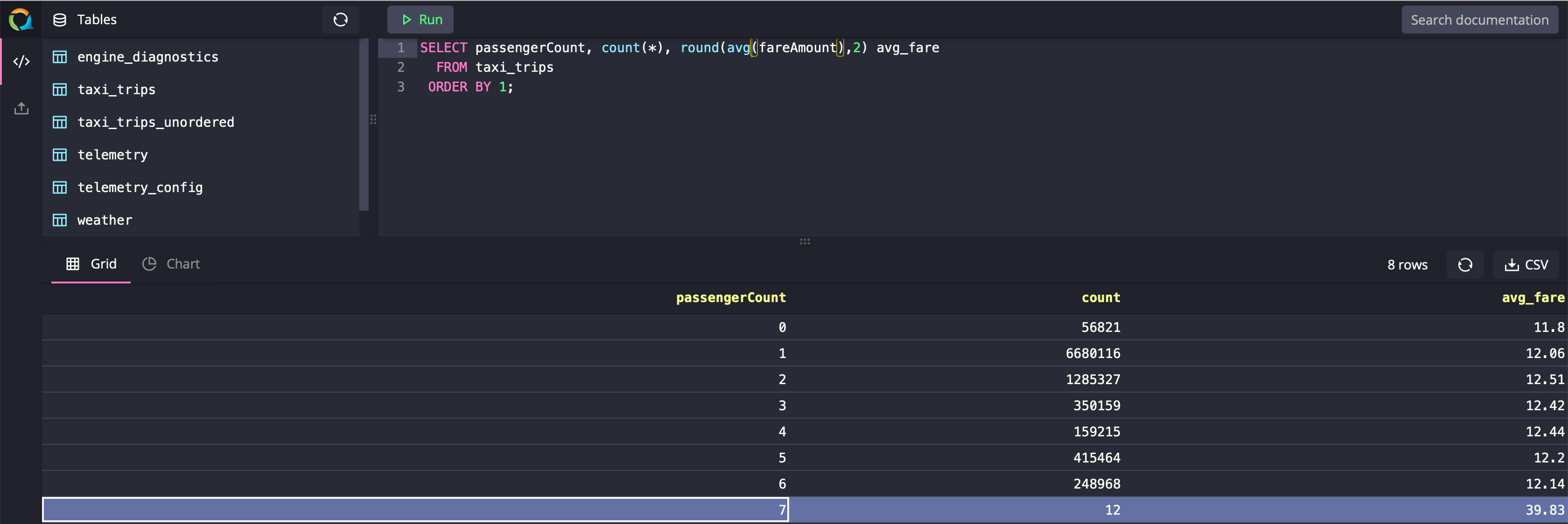
Optional GROUP BY Clause
Because of the widespread use of aggregation functions in the time-series databases, QuestDB implicitly groups the aggregation results to make the query writing experience better. While GROUP BY the keyword is supported by QuestDB, it would not make any difference to the result set if you include it in your query or not. Let’s see an example:
xxxxxxxxxx
SELECT passengerCount, COUNT(*), ROUND(AVG(fareAmount),2) avg_fare
FROM taxi_trips
ORDER BY 1;
SELECT passengerCount, COUNT(*), ROUND(AVG(fareAmount),2) avg_fare
FROM taxi_trips
GROUP BY passengerCount
ORDER BY 1;
Implicit HAVING Clause
As HAVING is always used only with the GROUP BY clause, HAVING clause automatically becomes implicit with an optional GROUP BY clause as mentioned above. Let’s see an example of this too:
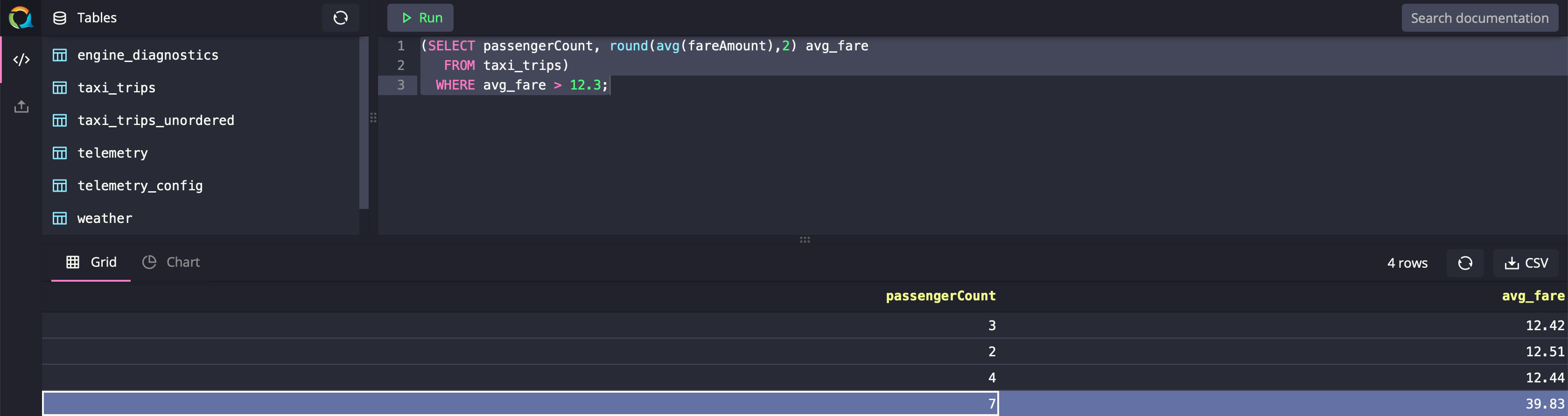
(SELECT passengerCount, round(avg(fareAmount),2) avg_fare
   FROM taxi_trips)
  WHERE avg_fare > 12.3;
Optional SELECT * FROM Phrase
QuestDB goes a step further by making the SELECT * FROM phrase optional. This one really helps reduce verbosity by a lot when there are nested subqueries involved. In QuestDB, just writing the name of the table and executing the statement will act as a SELECT * FROM TABLE_NAME statement. Please look at the example below:
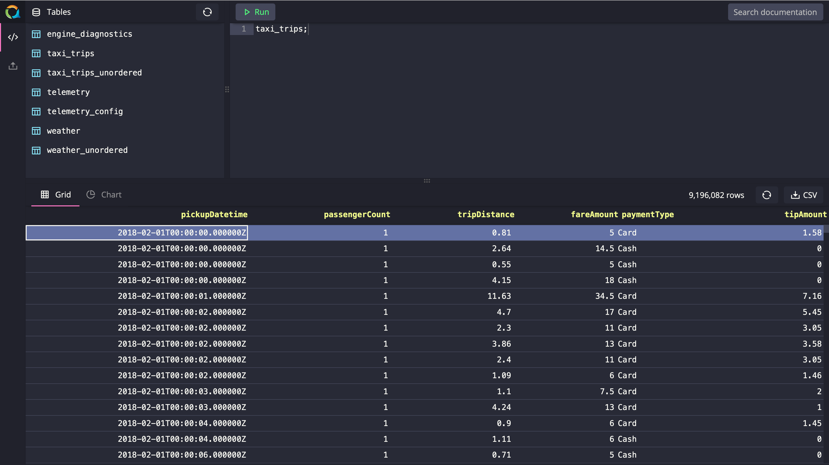
All of these improvements help reduce the effort required to write and maintain queries in a time-series database like QuestDB at scale.
Conclusion
In this tutorial, you learned how QuestDB supports SQL and enhances performance and developer experience by writing custom SQL extensions specially designed for time-series databases. You also learned about a few syntactical changes in QuestDB’s SQL dialect. If you are interested in knowing more about QuestDB, please visit QuestDB’s official documentation.
Published at DZone with permission of Kovid Rathee. See the original article here.
Opinions expressed by DZone contributors are their own.
Comments