Keep Calm and Column Wise
In this article, we’ll give you an overview of the challenges of implementing column-wise storage for JSON and the techniques used to address these challenges.
Join the DZone community and get the full member experience.
Join For FreeWhile SQL was invented for the relational model, it has been unreasonably effective for many forms of data, including document data with type heterogeneity, nesting, and no schema. Couchbase Capella has both operational and analytical engines. Both the operational and analytical engines support JSON for data modeling and SQL++ for querying. As operational and analytical use cases have different workload requirements, Couchbase's two engines have different capabilities that are tailored to address each workload's requirements. This article highlights some of the new features and capabilities of Couchbase's new analytical service, the Capella Columnar service.
To improve real-time data processing, Couchbase has introduced the Capella Columnar service. There are many differentiating technologies in this new service, including column-wise storage for a schemaless data engine and its processing. In this article, we’ll give you an overview of the challenges of implementing column-wise storage for JSON and the techniques used in the Columnar service to address these challenges.
Row-Wise and Column-Wise Storage of Data
Row-Wise Storage
With row-wise storage, each row of a table is stored as a contiguous unit within the table's data pages. All the fields of a single row are stored contiguously together, followed by the next row's fields, and so on. Each row can have 1 to N columns, and to access any one of the columns, whole rows are brought into memory and processed. This is efficient for transactional operations, as usually all or most fields are needed.

Figure 1: Logical table to physical row-wise representation
Column-Wise Storage
Column-wise storage, on the other hand, stores each column (a.k.a, field in a JSON document) of data separately. All values of a single column are stored contiguously. This format is particularly efficient for analytical and read-heavy operations that involve querying a few columns over many rows, as it allows for faster reading of relevant data, better compression, and more efficient use of resources like disk I/O requests.
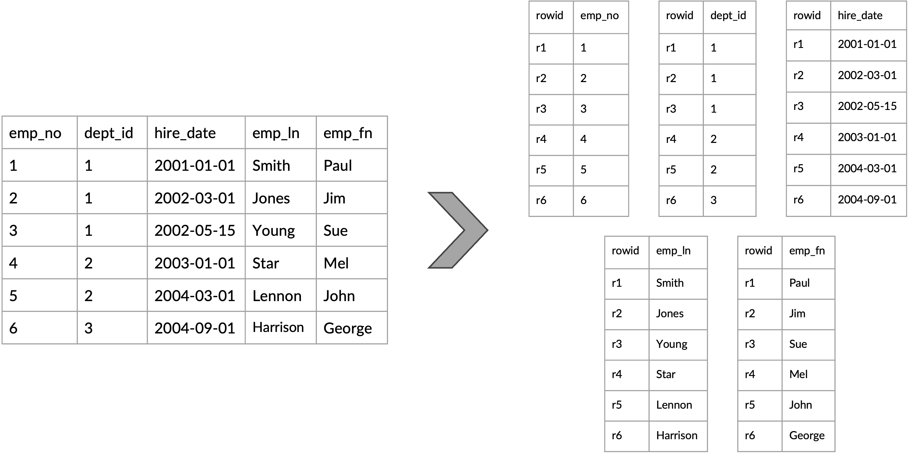
Figure 2: Logical table to physical column-wise representation
Document-Wise (Similar to Row-Wise) Storage
Each document of a collection is stored as a contiguous unit. This means that all the fields sub-fields of a single document are stored together, followed by the fields of the next document, and so on. This approach is efficient for transactional operations, as it allows for the quick retrieval of complete documents. However, it can be less efficient for analytical queries that access only a few fields across many documents, as unnecessary data from each document is also read.
With a JSON (document) data model, you typically have more fields in each document compared to a single row in a relational table. But, for analytical workloads, each query still reads a few fields from each document. So, the potential benefits of column-wise storage for a document store are even more than for relational databases. But, also, it’s not easy to implement! In flat relational tables, where the schemas are well-defined, and the columns' types are known a priori, the techniques used to store and query data of such tables are well understood. However, implementing a column-wise storage engine for a JSON document store is difficult since many of the things that make JSON ideal for modern applications make it difficult for column-wise storage! Here are the top reasons:
- Schema Flexibility
- Nested and Complex Structures
- Handling Heterogeneous Types
- Dynamic Schema Changes
- Compression and Encoding Challenges
Let’s look into each of these challenges briefly:
- Schema Flexibility: JSON is schema-less, meaning that each document is self-describing and can have a different structure with different fields. This flexibility is in stark contrast to the rigid, predefined schema of traditional relational databases. In a JSON model of customer documents, one record might have an address field, while another might not, in a distinct substructure, as in the example shown below. In a columnar database, this unpredictability makes it challenging to define a consistent column structure.
{
  "customer_id": 101,
  "name": "Alice Smith",
  "email": "alice.smith@example.com",
  "address": {
    "street": "123 Apple St",
    "city": "Wonderland",
    "zip": "12345"
  }
}

{
  "customer_id": 102,
  "name": "Bob Jones",
  "email": "bob.jones@example.com"
  // Note: No address field
}

{
  "customer_id": 103,
  "name": "James Brown",
  "email": "james.brown@example.com",
  "address": {
    "street": "Kenmare House, The Fossa Way",
    // First appearance of county
    "county": "County Kerry",
    // postcode instead zip
    "postcode": "V93 A0XH",
    // First appearance of country
    "country": "Ireland"
  }
}- Nested and Complex Structures: JSON supports arbitrary nested structures, like objects within arrays within objects. Columnar storage typically works best with flat, tabular data, and mapping these complex, hierarchical structures to columns can be extremely complex. As in the example shown below, a single JSON orders document may contain a list of items, and each item might have its own properties. Simply flattening this into columns would be challenging and could lead to a massive number of sparse columns. In our example below, the ordered item with an item_id = 1001 is the only one with the applicable promo code, and thus it is missing (akin to NULL in relational databases) in all other items.
{
  "order_id": 5002,
  "customer_id": 101,
  "date": "2023-11-24",
  "items": [
    {
      "item_id": 1001,
      "quantity": 1,
      "purchase_price": 1200.00,
      // The only item that has applicable promo code
      "promo": "BLACK-FRIDAY"
    },
    {
      "item_id": 1002,
      "quantity": 1,
      "purchase_price": 30.00
    }
  ]
}

{
  "order_id": 5003,
  "customer_id": 103,
  "date": "2023-02-15",
  "items": [
    {
      "item_id": 1003,
      "quantity": 1,
      "purchase_price": 80.00
    },
    {
      "item_id": 1004,
      "quantity": 2,
      "purchase_price": 300.00
    },
    {
      "item_id": 1005,
      "quantity": 1,
      "purchase_price": 99.00
    }
  ]
}- Handling Heterogeneous Types: JSON values can be of different types (e.g., strings, numbers, booleans, or even complex types such as objects and arrays). In a single field across different documents, the data type might vary, whereas columnar relational databases and even columnar file formats usually require all data in a column to be of the same type. If a 'price' field is sometimes stored as a string ("10.99") and other times as a number (10.99) or even as an array ([10.99, 11.99]) (assuming storing all seasonal prices), this complicates the process of storing and retrieving the data from a source that stores such data in a columnar format, where the data types are expected to be uniform.
{
  "item_id": 3003,
  "price": 10.99
}

{
  "item_id": 3004,
  "price": "10.99"
}

{
  "item_id": 3005,
  "price": [10.99, 11.99]
}

{
  "item_id": 3006,
  // price is missing (perhaps indicating unavailable or unknown price)
}- Dynamic Schema Changes: Because JSON is schema-less, the structure of the data can change over time. This flexibility is one of the attractions of JSON for modern applications. This could be problematic for columnar relational databases, where schemas do not change frequently. In schemaless document stores, however, adding new fields or even changing existing fields' simply works. For instance, an application might start capturing additional user data, such as customers' addresses, or changing the price from one data type to another. In a relational columnar database, this would require adding a new column, which could be a relatively heavy operation (especially in data warehouses) or not even possible in the case of changing a field's data type.
| Adding new field(s): Customers | Field's data type change: Items | |
|---|---|---|
| Before Upsert |
JSON
|
JSON
|
| After Upsert |
JSON
|
JSON
|
- Compression and Encoding Challenges: One advantage of columnar storage in a relational database is the ability to use very efficient encoding schemes, as values of the same types and the same domain are stored contiguously, and schemas are stored separately from data. However, the varied and complex nature of JSON can make it difficult to apply these effectively. For a purely numerical column, simple encoding and compression techniques can be very effective. But if a column mixes strings, numbers, nulls and missings (and even arrays and objects) in unpredictable ways, finding an efficient encoding strategy becomes much more complicated or even not possible.
Columnar Storage Engine in Capella Columnar
For its column-wise storage, Capella Columnar uses an extended version of the techniques and approaches described in this technical paper: Columnar Formats for Schemaless LSM-based Document Stores. You can find even more details in Wail Alkowaileet’s doctoral thesis, Towards Analytics-Optimized Document Stores. These techniques were originally implemented for Apache AsterixDB and are now part of Couchbase Capella Columnar.
Storage Overview
The columnar technology in Capella Columnar addresses the limitations of document store databases for analyzing large volumes of semi-structured data due to their inability to effectively use column-major layouts, which are, of course, more efficient for analytical workloads. The goal is to provide an efficient column store for JSON while retaining all the advantages of the JSON data model and improving query processing. In this part of the article, we describe the enhancements and improvements in these areas to overcome the challenges described earlier. See the aforementioned paper and thesis for further details.
The remainder of this article describes the following aspects of the new Capella Columnar Service offering:
- JSON data ingestion and columnization pipeline
- Columnar JSON representation
- Columnar storage physical layout
- Query processing for columnar collections
JSON Data Ingestion and Columnization Pipeline
Capella Columnar can ingest data from various data sources, such as the Capella Data Service, or from other external sources, such as other document stores and relational databases. Capella Columnar's storage engine is a Log-structured Merge tree (LSM)-based engine, and it works as illustrated in Figure 3. When JSON documents arrive at Capella Columnar from one of the supported sources, these documents are inserted into a memory component (also known in the literature as a memtable), which is a B+-tree stored entirely in memory. Once the in-memory component is full, the inserted documents are written to disk (via a flush operation) into an on-disk component (also known in the literature as an SSTable), which is a B+-tree fragment stored entirely on disk. The freed memory component can then be reused for a new batch of documents.
The batching nature of LSM provides an opportunity to "rethink" how the documents in the in-memory component should be written and stored on disk. In Capella Columnar, we take this opportunity to (1) infer the data's schema and (2) extract the values from the ingested JSON documents and store them into columns — both performed by the Columnar Transformer, as shown below in Figure 3. The inferred schema is used to identify the columns that appeared in those documents — more on that will be discussed later. Note that Capella Columnar performs both (1) and (2) simultaneously (i.e., in a single pass on each flushed JSON document). At the end of the flush operation, the inferred schema is persisted into the newly created on-disk LSM component to be retrieved when needed.

Figure 3: Data ingestion workflow
Columnar JSON Representation in Capella Columnar
Now that we know we have an opportunity to (1) infer the schema and (2) columnize the ingested JSON documents, the main question is: How can we represent those ingested JSON documents as columns and also allow them to be stored, updated, and retrieved — given the five challenges imposed by the JSON data model?
Capella Columnar represents ingested JSON documents using the approach described in this paper, which extends the Dremel format (introduced by Google in the paper Dremel: Interactive Analysis of Web-Scale Datasets) to address those five challenges. It is worth noting that Apache Parquet is an open-source implementation of the schema-ful Dremel format, and hence, without our extensions, it would not be possible to use Apache Parquet (as-is) in a document database. In the following, we describe how Capella Columnar represents the ingested JSON documents in a columnar layout using our extended Dremel format.
Let's start by taking a simple example of how to represent the first Customers JSON document from Listing 1, which is shown below in Figure 4.
|
Document
|
Inferred Schema
|
|---|---|
|
JSON
|
 |
| Data Columns | |
 |
|
Figure 4: Representing the first Customers JSON document as columns
First, we see that the schema is a tree structure that describes what is in the Customers document. Starting from the tree's root (a JSON object or document), we see that it has four children. The root's children represent the root's fields, which are customer_id, name, email, and address. Note that the address is also an object (or a sub-document) nested within the main document, and the object address has three children: street, city, and zip. We can see that scalar values are the leaves of the schema's tree structure — both for the root document and the address's sub-document. Each scalar value is assigned what we call a "column index." For example, the leaf 0:int tells us that the field customer_id – the collection's primary key (PK) – is an integer and is assigned the column index 0. Similarly, 4:string tells us the city value in the address object is of type string and is assigned the column index 4. From the schema, we can deduce that we have six columns (i.e., six leaves and each leaf is assigned a column index within the range [0, 5]).
So, the schema gives us a description of the document's structure and the types of values but not the values themselves. In Capella Columnar, the documents' values are stored separately from the schema as columns. Figure 4 shows the "Data Columns" (six columns, to be exact), and each column is represented as two vectors (depicted as a table with two columns in the figure for easier interpretation by the reader) called "D" and "V." The "D" vector in each column is what we call (as in Dremel) the Definition-level vector, and "V" is the Value vector. As can probably be inferred from the figure, the Value's vectors store the actual values from the JSON document. On the other hand, the Definition-levels's vectors are used as "meta-values" to determine whether a particular value is present or absent (i.e., NULL or missing). Let's take Column 1, which corresponds to the name field in our example. We see that the value "Alice Smith" has a definition level equal to 1, which tells us that this particular value of Column 1 is present, and its associated value is "Alice Smith." Now, let's take Column 4, which corresponds to the city in the address sub-document. It has a definition level equal to 2, and the value is "Wonderland." So, why is the definition level 1 in name and 2 in the city of the sub-document address? The definition level (as the name suggests) tells us at what (nesting) level a value appeared, given the inferred schema definition of this particular value. So, the name is a child of the root document. Thus, it is one level from the root, whereas the city is a child of the sub-document address, and hence, it is two levels from the root (root → name vs. root → address → city).
To better understand the handling of missing values, let's now add the following document:
|
Document
|
Data Columns
|
|---|---|
|
JSON
|
 |
Figure 5: Handling missing values
The schema is the same, as the fields that appeared in the document above (Figure 5) are a subset of the first document's fields shown in Figure 4; hence, no changes are required in the inferred schema. However, let's take a look at the Data Columns after adding the above document. We see that Column 1 (name) is also present in the second document, and its value is "Batman." However, Column 2 has a definition level equal to 0 in the second document, which tells us that the email field is missing for this customer. For the same customer, we see that both the street and zip are also missing, and hence, both Column 3 and Column 5 have a definition level equal to 1. However, Column 4 (city) is present (definition-level = 2) and the value is "Gotham". In Column 3 and Column 5, the parent sub-document is present (i.e., address) but not the street and zip values. Note that having the definition level equal to 1 in both Column 3 and Column 5 is not required to deduce that the address is not missing. Since Column 4 (city) is present, it implies that its parent (address) is also present. That is, both Column 3 and Column 5 can have a definition level of 0, and we can still reassemble the document to its original form without any loss. Therefore, we can say that the address itself is missing if we have the definition levels for street, city, and zip equal to 0.
As explained above, the definition level determines whether a value is present or not. However, it serves a different purpose for primary keys' (PKs) columns. The definition level in a PK distinguishes an actual JSON document from an antimatter (or tombstone) entry. Since PK fields cannot be missing, the definition levels of the PK values are used to distinguish antimatter entries, which have no values in any of the non-key columns, from actual JSON documents (non-antimatter), which can have any number of values in non-key columns. We omit the technical details here of handling antimatter entries (the details are in the paper). However, it is important to note that the ability to handle antimatter entries allows Capella Columnar to perform deletes and upserts against collections that are stored using this columnar representation.
Schema Flexibility and Dynamic Schema Changes
In the previous example, we show that fields in any documents can be missing (i.e., they are optional) – except for the primary keys. Also, in the previous example, the first document's schema was a superset of the second document's schema. Hence, the schema did not need to change when we added the second document. However, to see how the schema can evolve, let's flip the order in which the two documents are processed and added, such that we can observe the case of inferring new columns in our columnar representation. Below, in Figure 6, we see that the first inferred schema contains only three columns: customer_id, name, and city (in the sub-document address), and we see their assigned column indexes of 0, 1, and 2, respectively. After adding the second document, three additional columns are added, namely email in the root document and street and zip in the address sub-document. Note that the newly added columns have the column indexes 3, 4, and 5 for email, street, and zip, respectively. The definition levels are exactly the same as in the previous example. The only change between the two examples (i.e., in Figure 6 vs. the one in Figure 5) is the column's indexes, but the rest is the same.
| After adding document with customer_id: 201 | After adding document with customer_id: 101 |
|---|---|
 |
 |
 |
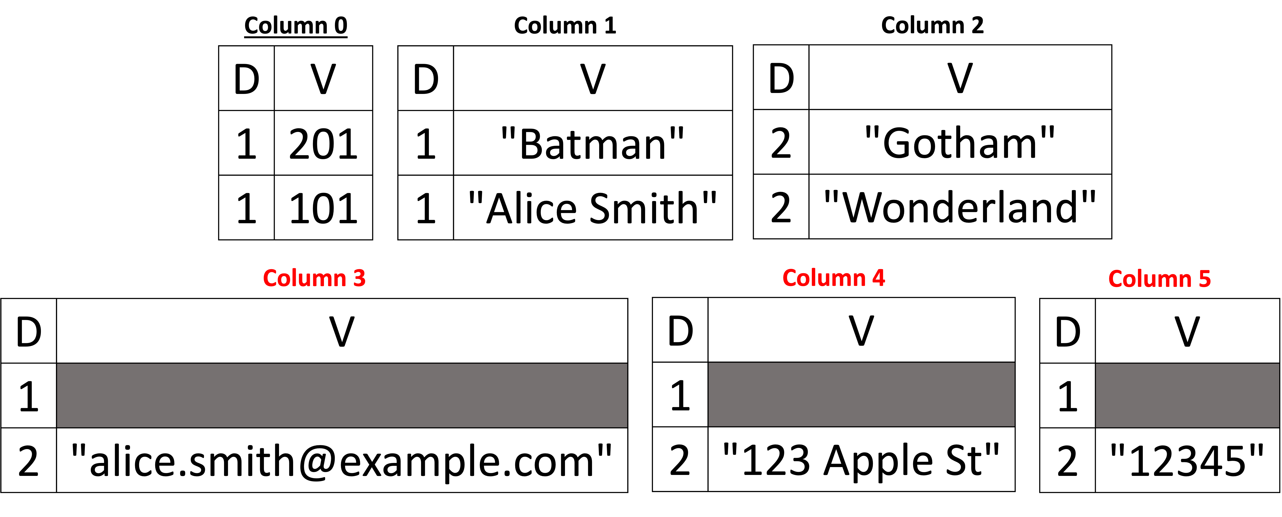 |
Figure 6: Handling schema changes
It is worth noting a technical detail here. We see that when we added a new column that belongs to a nested field (for example, Column 5, which corresponds to zip), the first definition level is 1, which corresponds to the missing zip value in the first document. But how did we get this information (i.e., the definition level is 1 but not 0 while we are adding a second document)? The parent can maintain a list of integers of all previous documents whose sub-document address was present or missing (i.e., the definition levels of address, which can either be 0s or 1s in all previous documents). When a new column is added, we first set the definition levels of the parent sub-document address to the newly created column. In our example, the address was present in the document with customer_id = 201. Hence, the address has a definition level of 1. When Column 5 was created, we added the definition level of 1 first to say the address was present in the previous document, but the value of the zip was missing. Maintaining this list in each nested node is optional for the reason explained above (we can simply add 0s for each newly created column). However, maintaining this list in memory can be relatively cheap using an appropriate data structure. In Capella Columnar, we implemented a simple data structure that exploits the reparative nature of the definition levels – and our experiments showed that it has a negligible memory footprint. Additionally, this integer list is bounded by the number of documents on each physical page, which is bound to 15,000 at most (see the paper for more details about this limit). Maintaining the actual definition levels of the parents' nodes simplifies the JSON document assembly algorithm (hence, better and easier maintainability of the document assembly code). Thus, we opted to do this in Capella Columnar.
Handling JSON Arrays
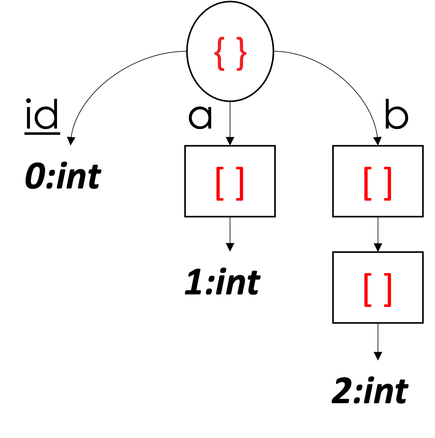
In the previous examples, we dealt with JSON objects (documents and sub-documents). Next, we focus on handling JSON arrays. Let's start with the simple example shown below in Figure 7. In this example, we have three documents, and from the schema, we can see that all documents have the field id, which is the primary key. The first two documents have two additional fields, a and b, where a is an array of integers and b is an array of arrays of integers. In the last document, both a and b are missing.
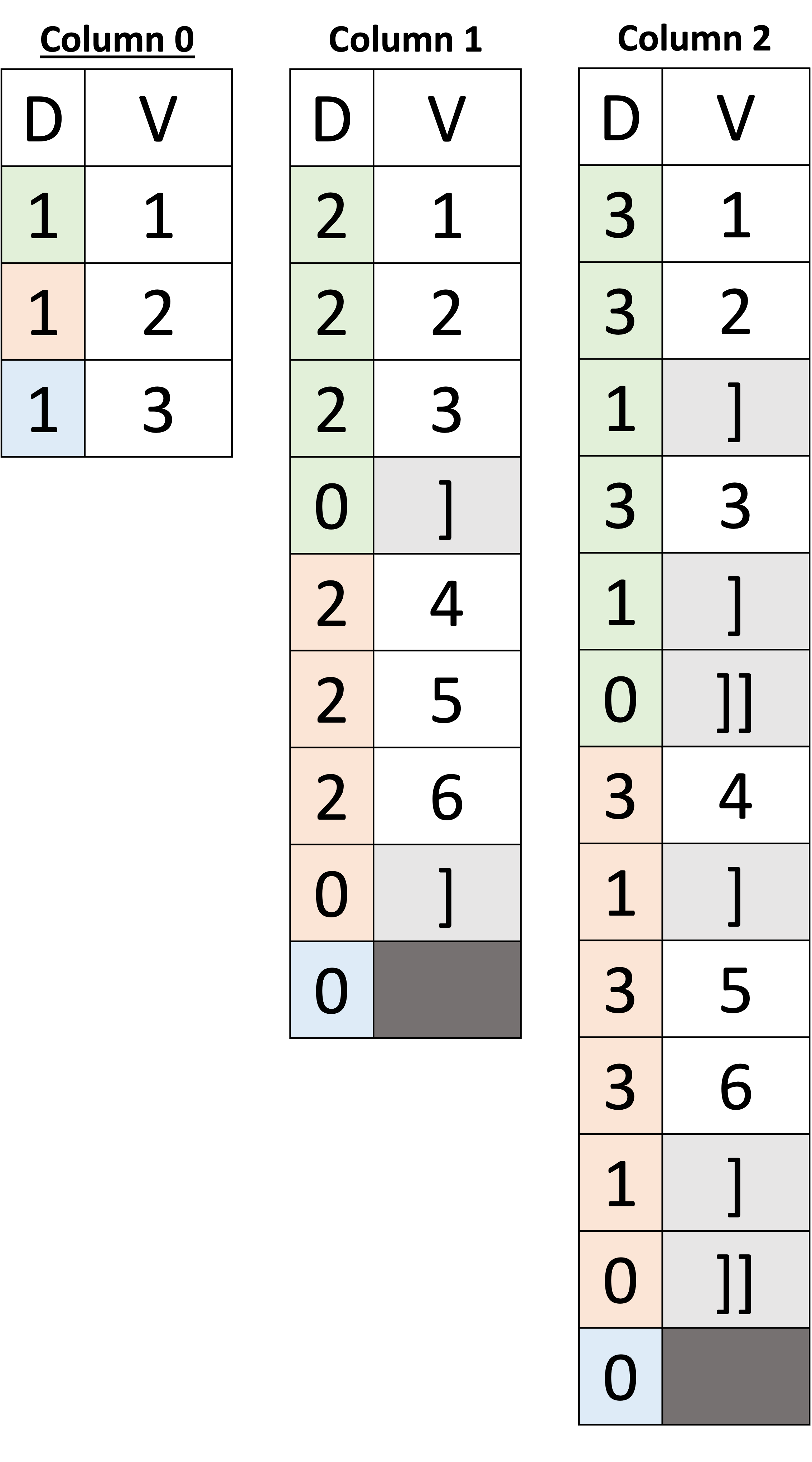
Starting with id, we can see that its values are stored in Column 0. In this example, we have color-coded the definition levels so that we can visually associate a value in a column with its document such that the greens belong to the first document, oranges belong to the second document, and sky-blues are for the third document. Hence, the ids 1, 2, and 3 in Column 0 belong to the first, the second, and the third documents, respectively.
Next, Column 1 stores the integer values of the array a for all three documents. The question now is how we can determine which value in this column belongs to which document. Using color coding, you can observe that the first four values belong to the first document – but how can a machine determine that? We can see that the array a in the first document has three integers [1, 2, 3], and each has a definition level equal to 2 (saying the values are present – as we saw earlier) followed by a definition level of 0. In the previous examples, we used definition levels to determine whether a value is present or absent. In arrays, definition levels have an additional role, which is acting as array delimiters; thus, after the first three definition levels (2, 2, and 2), the last definition level (0) is a delimiter, which tells us that the end of the array has been reached, so the following value belongs to the next document. Note that we put ']' in the Value vector; however, this is for illustration purposes only – array delimiters do not have any value. As in the first document, the following definition levels in orange (2, 2, and 2) indicate the presence of the second document's values of the array a, and the values are [4, 5, 6]. Again, the following definition level of (0) indicates the end of the array for the second document. Following the delimiter of the second document, we see a sky-blue definition level of (0), which corresponds to the third document, where the array a is missing. Hence, the definition level of (0) indicates that the array a is missing in the third document – why is it not a delimiter, you may ask? A definition level can be interpreted as a delimiter if an array element is observed as present a priori; otherwise, it is an indication of a missing value. In other words, a delimiter must be preceded by a value with a higher definition level; otherwise, the observed definition level is an indication of a missing value and not an array delimiter.
|
Documents
|
Inferred Schema
|
Data Columns
|
|
|---|---|---|---|
|
JSON
|
 |
 |
|
Figure 7: Representing JSON arrays
Now, let's see how an array of arrays (such as b in Figure 7 above) is represented. Simply by looking for the delimiters in Column 2, which are marked as ']' for inner and ']]' for outer, we can see there are two delimiters with two different definition levels: 1 and 0. In Column 2, we need two delimiters to distinguish the inner and the outer delimiters. For instance, after the values [1, 2] in the first document, a delimiter with the definition level 1 is placed, indicating the end of the inner array, followed by the value [3], which indicates the first element of the second inner array. After the value [3], we see two consecutive delimiters with definition levels 1 and then 0. The first delimiter with the definition-level 1 tells us the end of the inner array, and finally, the delimiter with the definition-level 0 tells us the end of array b in the first document – hence, the following value belongs to the second document. Similarly, for the second document, we have the value [4] followed by a delimiter with definition-level 1 – indicating the first inner array has only a single element [4]. Then, we have the values [5, 6] followed by the delimiters with definition levels 1 and then 0 – indicating the end of the second inner array and the outer array, respectively. Finally, the definition-level 0 in the third document indicates that the array b is missing.
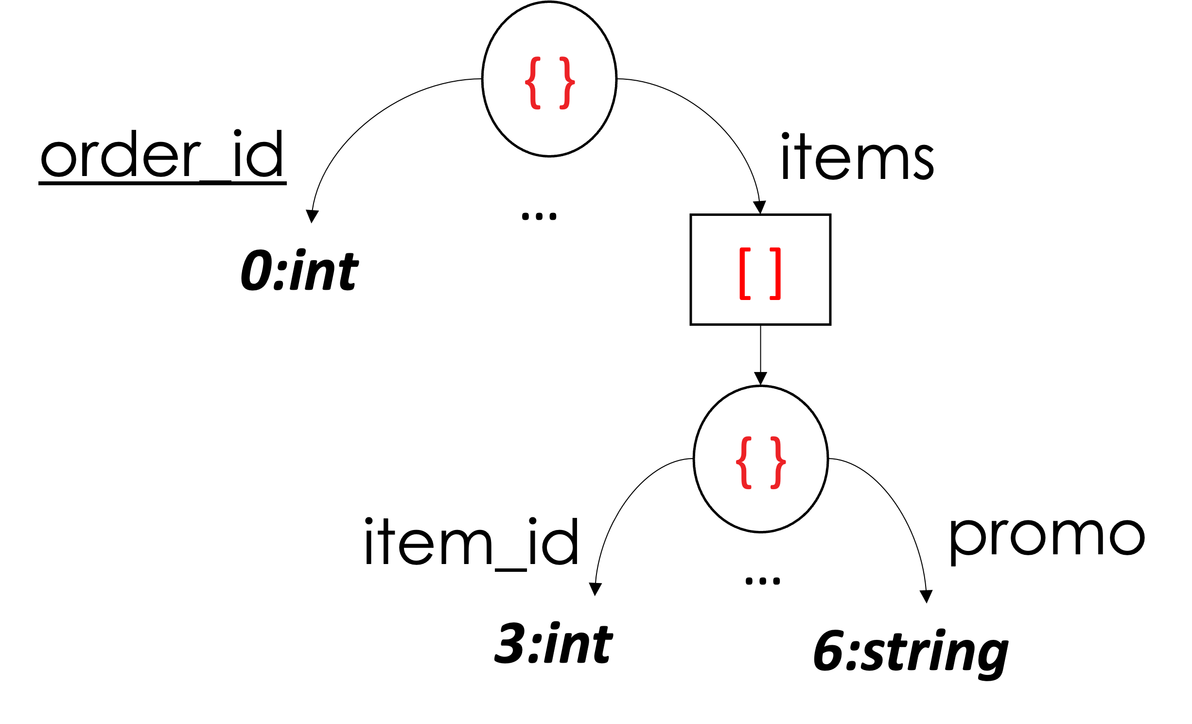
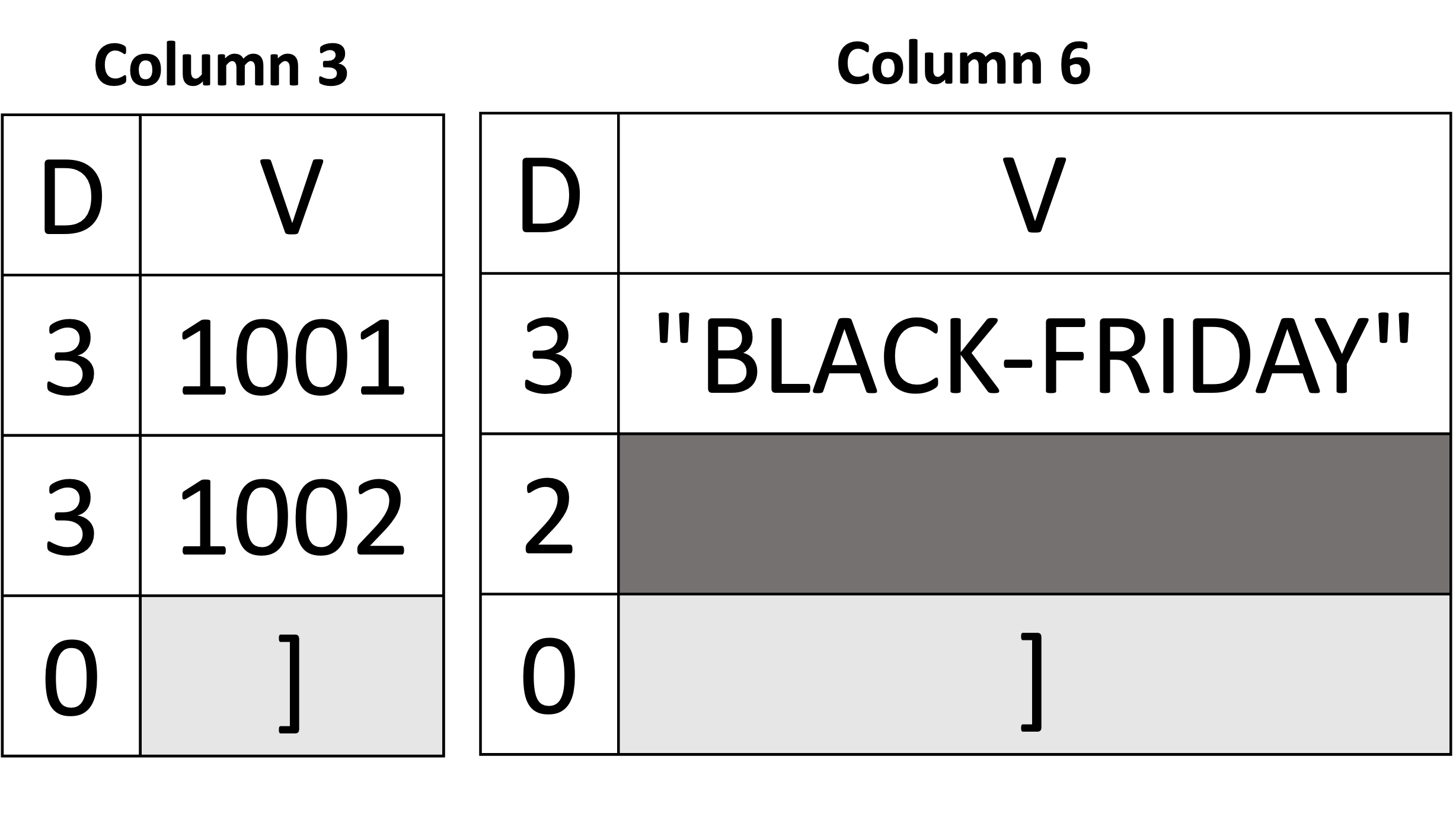
That's it for representing an array and an array of arrays of scalar values! Next, we explain the representation of an array of objects. Let's start with the example shown below in Figure 8 using the first Orders document in Listing 2. The example only shows two columns (out of six) and omits the rest (the omitted ones can be used as an exercise for the reader). Mainly, we will focus on Column 3 and Column 6 (i.e., item_id and promo from the schema). Both columns belong to the same array items. From a "column perspective," it "sees itself" as an array of scalar values. In other words, we can see the values of item_id as an array of integers [1001, 1002] and the values of promo as an array of strings ["BLACK-FRIDAY," missing]. Thus, representing an array of objects can be seen as representing two different scalar arrays with the same number of elements. Consequently, they will have their delimiters exactly at the same position. In our example below, the array delimiters of both Column 3 and Column 6 appear exactly at the 3rd position. Another distinction (compared to an actual array of scalars) is at which definition-level a value is present. Since both columns are descendants of the same array of objects, a definition level equal to 3 is an indication of a present value – as the values of both item_id and promo appeared at the third level from the root. E.g., root (0) →\rightarrow→ items (1) →\rightarrow→ object (2) →\rightarrow→ promo (3). When we reassemble the columns back to their original form, we can see that there are two objects in the array items, where item_id is 1001 in the first object and 1002 in the second. Similarly, the promo is "BLACK-FRIDAY" in the same first object and missing in the second.
|
Documents
|
Inferred Schema
|
Data Columns
|
|
|---|---|---|---|
|
JSON
|
 |
 |
|
Figure 8: Representing an array of objects
Handling Heterogenous Types
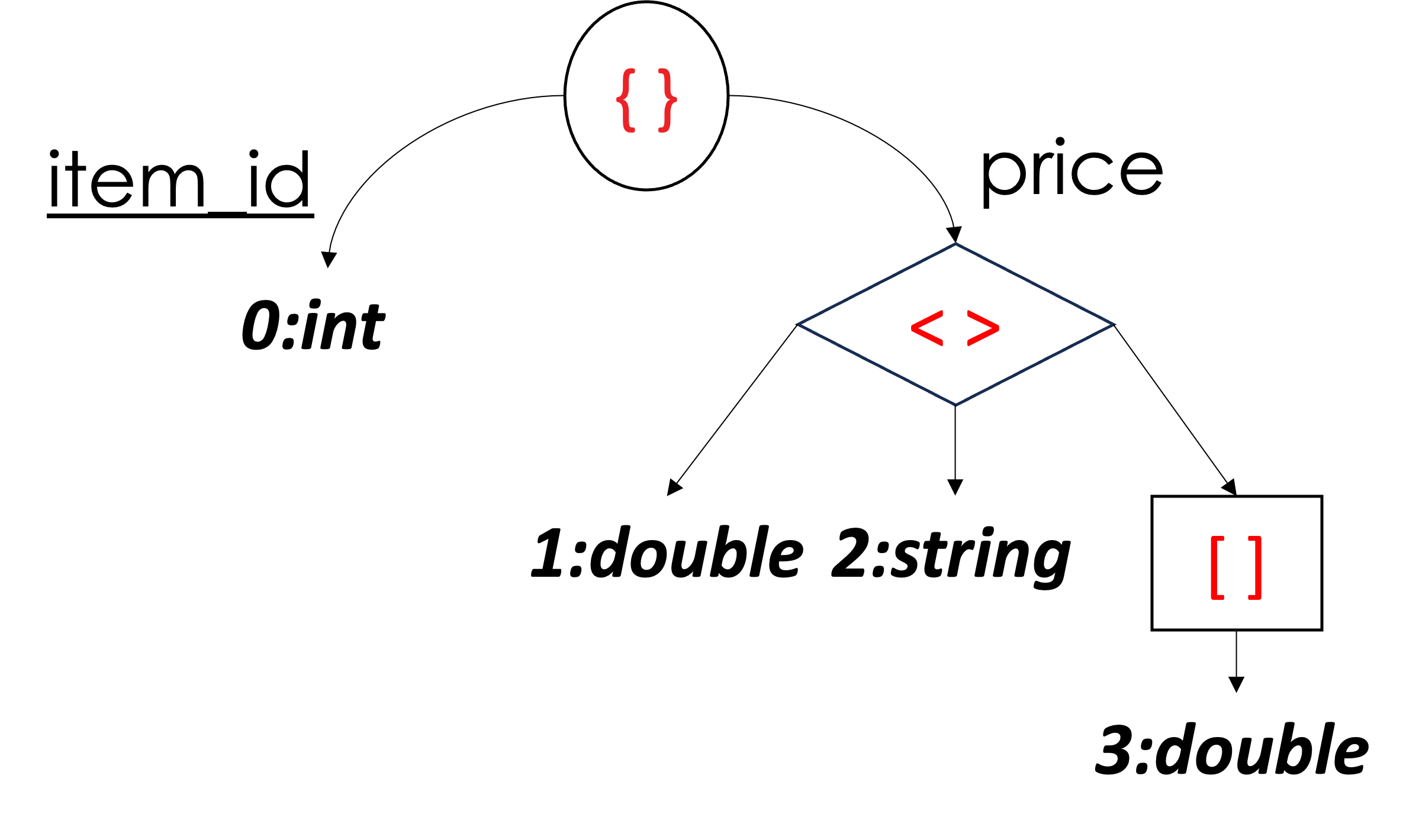
Alright! Up to this point, we know how to represent JSON objects, arrays, and their scalar values as columns and how to handle schema changes (i.e., inferring new columns). Next, we explain how to handle heterogeneous data types. Let's take the example shown below in Figure 9 using the documents shown in Listing 3. First, we see that we have four documents where the field price can be either a double, a string, an array of doubles, or a missing value. The inferred schema represents the type of price as a union of either double, string, or array. A union node in the schema tree structure is represented as a diamond in Figure 9, with three children. Union types in the inferred schema are a special case in three ways. First, a union is a logical description that cannot exist in an actual document. Second, since it is a logical description, it does not affect the definition level. Third, only a single value can be present in a union value, and the rest must be missing — and when all values are missing, then the union value is itself indicated as missing.
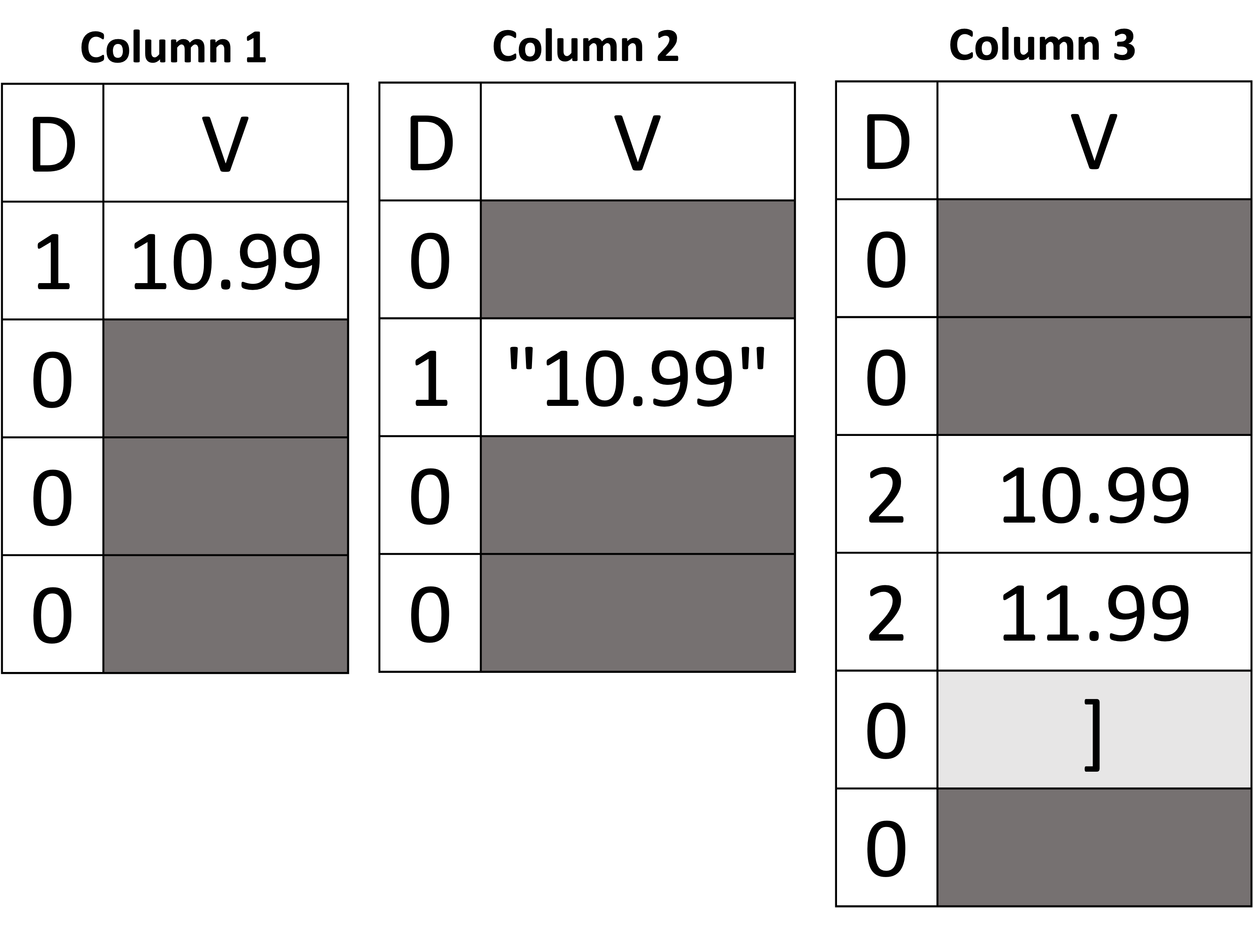
Let's unpack this and use the example below to understand those three criteria of a union type. First, we see that Column 1, Column 2, and Column 3 all belong to price. As in a sub-document, the branches of a union can have any number of columns. For instance, Column 1 corresponds to the double-type version of price, Column 2 is the string-type version of price, and Column 3 is the array-of-doubles-type version of price. When the value price is accessed, all three columns must be read at the same time to determine the actual value of the price. Starting with Column 1, we see that the first value has a definition level equal to 1, which indicates that the value is present and its value is 10.99. Note that having the union between the root and the column itself did not change the result (i.e., the result is still double as shown in the first document – the 1st criterion from above). Also, note that the definition level is 1 (not 2) even though the path from the root to Column 1 goes through the union node (the 2nd criterion). Now, since Column 1 contains a non-missing value for the first document, the values in Column 2 and Column 3 for the same document are missing (the 3rd criterion). In the second document, the price is a string. Hence, the string value is present in Column 2, and both Column 1 and Column 3 are missing. In the third document, price is an array of doubles, and hence, the array's values for price are stored in Column 3. Finally, in the fourth document, the field price is missing. Therefore, the definition level is 0 in all three columns – indicating that the price itself is missing.
| Documents | Inferred Schema | Data Columns | |
|---|---|---|---|
|
JSON
|
 |
 |
|
Figure 9: Representing heterogeneous types
Encoding
In this representation, we see that each column stores values that are all of the same type and domain. Even in fields with heterogeneous data types like price in Figure 9, each physical column is dedicated to storing one specific data type of the price values. This gives us the opportunity to use the same efferent encoding schemes used in Parquet, currently excluding dictionary encoding (due to its requirement for additional storage pages). We are planning to explore the potential benefits/drawbacks of including dictionary encoding in a future release.
We now see that Capella Columnar – using this columnar representation – is capable of handling the flexibility of schemas in the JSON data model, as well as handling dynamic schema changes when storing the data as columns. Also, the representation is capable of handling the nested nature of the JSON data model. Finally, the schema and columns can adapt dynamically when encountering heterogeneous value types.
Columnar Storage Physical Layout
Since we know how to represent JSON documents as columns, the question now is how to actually store them. Earlier, we described the ingestion pipeline in Capella Columnar, and we explained how the JSON documents are written as columns into on-disk LSM components. So, let's dive in and see what is inside an on-disk component. An on-disk component is a B+-tree stored entirely on disk. In Capella Columnar, we use the physical storage layout described in the paper, known as AsterixDB Mega Attributes across (or AMAX), to store the data columns. Figure 10 depicts the storage layout. Each AMAX LSM component is also a B+-tree; however, the leaf nodes of the B+-tree are mega-leaf nodes, each of which can occupy multiple data pages instead of a single data page, as in the original B+-tree. In Figure 10, we see that there are four mega leaf nodes (four arrows coming from the interior nodes), each of which occupies a different number of data pages. Zooming in on one of the mega leaf nodes, we see that it consists of 5 data pages (page 0 to page 4). Page 0 is a special page, as it stores the mega leaf node header containing meta information about the mega leaf node. Additionally, Page 0 stores all of the mega leaf nodes' primary keys, as well as fixed-length prefixes of the minimum and maximum values for each column, which can be used to filter out mega leaf nodes when an LSM component is queried (more on that later).
Next, Pages 1 to Page 4 store the columns' data (namely their definition levels and their values). In the same figure, we see some logical representations called Megapages, each of which stores the data for a specific column. For instance, megapage 1, which occupies page 1, page 2, and part of page 3, stores the data for a single column. The same goes for megapage 2, which occupies page 3 and page 4, and which stores another column's data.

Figure 10: Columnar storage physical layout (AMAX)
Query Processing Techniques for Columnar Collections
When an LSM component for a collection's primary index is queried, each mega leaf node in the B+-tree in Figure 10 above is processed (left-to-right). However, only the relevant megapages (or columns) will be accessed in each mega leaf node. For example, suppose that the following query is executed:
SELECT AVG(i.price)
FROM Items i
In each mega leaf node, only Page 0 will be accessed along with the mega page that corresponds to the price value (or column). For instance, let's say that megapage 2 stores the price values; then only Page 0, Page 3, and Page 4 will be accessed, and Page 1 and Page 2 will be skipped – reducing the I/O cost.
As we mentioned, Page 0 also stores fixed-length prefixes of the minimum and maximum values for each column. Let's say that we want to run another query such as the following:
SELECT *
FROM Customers c
WHERE address.city = "Gotham"
When a mega leaf node is accessed, the first page we read is Page 0. So, before reading the other pages required by a query (in the case of the query above, it is all the columns), we use the filters in Page 0 to skip reading the mega pages of a mega leaf node when the min/max filters cannot satisfy the condition address.city = "Gotham". Hence, a number of mega-leaf nodes can be skipped. Such filters can accelerate the execution of a query significantly if the filter is selective.
The query above does SELECT *, which requires assembling the JSON documents back to their original form. The assembly cost – a CPU cost – can be high if the number of columns is high. To avoid paying unnecessary costs, Capella Columnar will push the WHERE-clause's predicate down to the storage layer. More specifically, what Capella Columnar does is that it first reads the columns required to evaluate the WHERE-clause in a query and postpones reading the other columns. When Capella Columnar finds a JSON document that satisfies the WHERE-clause's condition, it then reads the other columns and only assembles the JSON documents that will satisfy the query condition. This approach of second-level filtration can act as a "second line of defense" when the range of the min/max filter on Page 0 is too "wide." Also, the cost of the reassembly is reduced by avoiding assembling JSON documents that do not satisfy the executed query's condition.
The aforementioned techniques work for a variety of queries. For instance, Capella Columnar's compiler can detect and use the filters even against array items, as in the query below:
-- Return the number of orders that contain at least one purchased
-- item with a purchase price less than 10.0
SELECT COUNT(*)
FROM Orders o
-- o.items is an array in Orders (see Listing 2)
-- The filter will be pushed and applied in
-- the storage layer even against array items
WHERE (SOME i IN o.items SATISFIES i.purchase_price < 10.0)
Finally, Capella Columnar also supports creating and using secondary indexes on columnar collections (as traditionally done for row collections) for further filtration.
Conclusion
Couchbase Columnar service is designed to provide a zero-ETL approach to bringing a wide variety of data into a single platform for real-time analysis. Its JSON data model, its efficient storage engine, and its query compiler and query processor are among the secret key ingredients for this recipe. Now you know the secret!
References
Opinions expressed by DZone contributors are their own.

Comments