Stop Loading Everything into Redshift: A Spectrum + Iceberg Pattern for Hybrid Analytics
Store large and cold datasets in Iceberg on S3, query them through Spectrum, and reserve Redshift local tables for workloads that need low latency or high concurrency.
Join the DZone community and get the full member experience.
Join For FreeNot every dataset belongs fully inside the warehouse. A hybrid design using Apache Iceberg on S3, Redshift Spectrum, and Redshift local tables can reduce duplicated storage and reserve warehouse performance for the workloads that need it.
The Warehouse Became the Second Data Lake
Redshift clusters routinely carry tables that should not be there. A five-year transaction history is loaded nightly through a four-hour COPY job and queried twice a quarter. Raw event tables landed directly into the warehouse because the lake pipeline was harder to set up. Aggregations that nobody owns, kept around because deleting them feels risky.
The pattern builds quietly. Once Redshift becomes the default destination, every new dataset gets a COPY job and a table definition. Storage compounds. Load windows stretch. The lake stays alive in parallel but loses authority over the data, while the warehouse takes on a role it was never priced for.
The hybrid pattern fixes the destination problem at ingestion time. Apache Iceberg on S3 holds curated and historical data. Redshift Spectrum exposes that data through external schemas, so the warehouse can query it without copying it. Redshift local tables stay reserved for workloads where sort keys, distribution, and result caching pay off.
The goal is not to move everything out of Redshift. The goal is to stop loading everything into Redshift by default.
The Decision Framework
The most useful question is not, “Can this dataset be loaded into Redshift?” In most cases, the answer is yes. The better question is, “Does this dataset deserve Redshift local storage?”
| data pattern | better fit | why |
|---|---|---|
| Hot dashboard data with sub-second SLAs | Redshift local | Sort keys, distribution keys, and result caching matter. Spectrum cannot reliably match local-table latency under concurrency. |
| Large historical data with infrequent reads | Iceberg + Spectrum | Storage cost dominates. Latency tolerance is higher. COPY duplicates a rarely touched dataset. |
| Raw or semi-curated landing data | Iceberg on S3 | Schema still drifts. Loading into Redshift forces premature contracts. |
| Aggregated daily or monthly marts | Redshift local | The footprint is usually small, query frequency is high, and joins against dimensions are common. Spectrum adds latency variance with little upside. |
| Backfill-heavy datasets | Iceberg + Spectrum | Snapshot rewrites are cheaper than repeated COPY cycles. Time travel and rollback come with the format. No COPY window blocks analysts. |
| Ad hoc exploration on wide event tables | Iceberg + Spectrum | Most queries scan a subset of columns. Parquet projection and external access keep duplicated storage under control. |
Two axes drive the decision: query frequency and latency tolerance. Size is secondary. A 50 GB table queried every minute with sub-second SLAs belongs in Redshift local. A 5 TB table queried weekly with a 30-second tolerance belongs in Iceberg. Teams that lead only with size often place the data in the wrong layer.
Default new datasets above a few hundred gigabytes to the Iceberg curated layer. Promote them into Redshift local storage only when a specific serving requirement justifies the duplication. Reverse migration rarely happens once data lives in the warehouse, so the default matters.
The Architecture
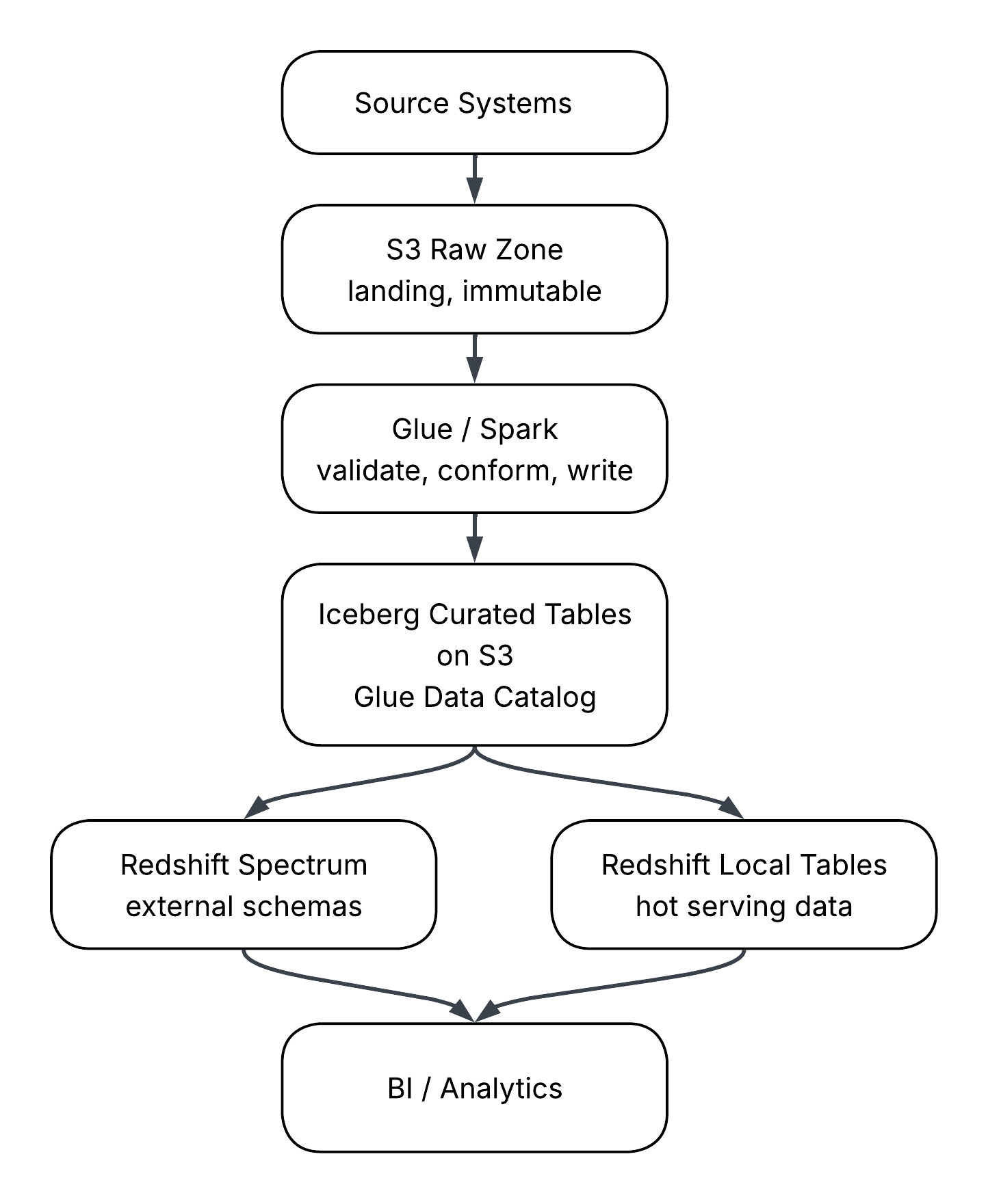
The flow is single-direction. Source systems land in an S3 raw zone. Glue or Spark jobs read raw data, apply schema and quality checks, and write to Iceberg tables in a curated zone on S3. Iceberg becomes the system of record for curated data.
From there, two consumption paths diverge. Redshift Spectrum reads Iceberg tables through external schemas registered against the Glue Data Catalog. A smaller set of high-value serving tables is materialized into Redshift local storage through scheduled COPY or INSERT jobs. BI tools and analyst queries hit Redshift, which routes the scan to local storage or Spectrum based on the schema referenced in the query.
A few things about this layout matter more than they look.
The Iceberg curated layer is the authoritative copy. Redshift local tables are derivatives. When a serving table in Redshift drifts from its Iceberg source, the Iceberg version wins, and the local table gets rebuilt. This rule prevents the slow split-brain that happens when teams patch warehouse tables directly while the lake quietly falls behind.
There are no back arrows for authoritative curated data. Redshift can write results back to S3, and current Redshift capabilities also include writing to Iceberg tables registered with the Glue Data Catalog. That does not mean the warehouse should become the producer of curated lakehouse data. In this pattern, curated tables come from the Glue or Spark layer. Warehouse-generated outputs are derivatives, exports, or serving artifacts, not authoritative sources.
The Glue Data Catalog is the contract surface. Spectrum reads schema and partition information from the catalog, not from S3 directly. That makes the catalog part of the analyst query path, not just a passive metadata store. Treat it accordingly: version table definitions, restrict who can alter schemas, and monitor for drift between catalog metadata and the underlying files.
Promotion from Iceberg to Redshift local storage is a deliberate step, not a default. The trigger should be a documented serving requirement: a dashboard SLA, a known concurrency pattern, or a join that Spectrum cannot execute fast enough. Without that trigger, the data stays in Iceberg, and Spectrum serves it.
The architecture does not solve placement by itself. It works only when the framework above is applied consistently at ingestion time.
Why Loading Everything into Redshift Becomes Expensive
The obvious cost is storage. The less obvious cost is the operating model created around that storage.
RA3 does not remove this design question. Redshift Managed Storage separates compute and storage and can scale warehouse storage independently, but the data is still a Redshift-managed copy with warehouse-side ingestion, permissions, lifecycle, and maintenance. RA3 changes the economics of storage growth. It does not make every lakehouse dataset a good Redshift local table.
When a dataset is copied from S3 into Redshift, the team now owns two versions of the same data. One version lives in the lake. Another version lives in the warehouse. If both are treated as durable assets, the platform has to answer a basic question every time a number does not match: which copy is correct?
That question is expensive because it creates investigative work. The difference may come from a delayed COPY job, a failed backfill, a schema mismatch, a stale warehouse table, or a manual patch. The data itself may be fine. The duplication is what makes the answer hard to trace.
Daily load jobs add another cost. A nightly COPY pattern feels harmless when the dataset is small. As history grows, the same job starts consuming more time, more warehouse capacity, and more engineering attention. Eventually, the load window competes with analytics workloads. Teams respond by tuning schedules, splitting files, adding staging tables, and building retry logic around data that may not need to be in Redshift at all.
Backfills make the problem worse. In a lakehouse pattern, a corrected Iceberg snapshot can become the new curated version. In an all-warehouse pattern, the correction often requires deleting, reloading, validating, and reconciling Redshift tables.
A simple rule helps:
| question | if yes | if no |
|---|---|---|
| Is this dataset queried daily or hourly? | Consider Redshift local | Keep in Iceberg and expose through Spectrum |
| Does it support a dashboard SLA? | Consider Redshift local | Avoid default duplication |
| Does it change frequently due to backfills? | Keep in Iceberg | Redshift local may be acceptable |
| Is it mostly historical or exploratory? | Keep in Iceberg | Evaluate serving needs |
| Does it require heavy joins under concurrency? | Consider Redshift local or pre-aggregated marts | Spectrum may be sufficient |
Redshift cost problems rarely start with one bad table. They start when every table receives the same answer.
The Spectrum + Iceberg Pattern in Practice
The practical pattern is simple: register the Iceberg curated tables in the Glue Data Catalog, create an external schema in Redshift that points to that catalog, and let analysts query external tables when the data does not justify local storage.
One caveat matters before standardizing on this pattern. Spectrum's Iceberg support has improved, but it should still be validated against the table format, write engine, and access pattern used in the platform. Redshift supports querying Iceberg tables cataloged in Glue and supports both Iceberg format versions 1 and 2, but feature behavior has continued to evolve across Redshift releases. Time travel queries are not currently supported for Iceberg tables through Redshift. Performance depends on Glue column statistics, metadata handling, and the table's physical layout. AWS recommends generating Glue column statistics for Iceberg tables as a prerequisite for good Spectrum query performance, not an optimization step. Treat the first implementation as a compatibility test, not only a SQL wiring exercise.
A simplified external schema setup looks like this:
CREATE EXTERNAL SCHEMA lakehouse_curated
FROM DATA CATALOG
DATABASE 'curated_iceberg'
IAM_ROLE 'arn:aws:iam::123456789012:role/redshift-spectrum-role'
REGION 'us-east-1';
After the schema is available, analysts can query external tables from Redshift:
SELECT
    event_month,
    product_line,
    COUNT(*) AS event_count,
    SUM(transaction_amount) AS total_amount
FROM lakehouse_curated.customer_events
WHERE event_month >= DATE '2025-01-01'
  AND event_month < DATE '2025-04-01'
  AND product_line = 'brokerage'
GROUP BY
    event_month,
    product_line;
The query looks like a normal SQL query, but the physical behavior is different. Redshift is not scanning local blocks. Spectrum is reading files from S3, using metadata from the Glue Data Catalog, and returning results back into the Redshift query. Performance depends heavily on file layout, partition pruning, column projection, and how much data Spectrum has to scan.
Iceberg helps because it brings table semantics to data stored on S3. It supports schema evolution, snapshot isolation, partition evolution, hidden partitioning, and time travel when accessed through engines that support it. Those features make the lakehouse layer safer to use as an authoritative, curated store.
Partitioning deserves special attention. Many teams treat partitioning as a folder layout problem. They choose obvious folder keys such as year, month, day, region, or source system, then assume the query engine will do the right thing. That works only when query filters line up with the partition design.
Naive partitioning can hurt Spectrum. A table partitioned too narrowly can create many small files and too much metadata overhead. A table partitioned on the wrong column can force wide scans even when the analyst's query appears selective. A table partitioned by ingestion date may perform poorly when analysts filter by business date.
Iceberg hidden partitioning reduces some of this pain because the table can define partition transforms without exposing physical partition columns directly to users. For example, an Iceberg table can partition a timestamp by day or month while analysts continue filtering on the timestamp column.
A conceptual Iceberg write might look like this in Spark:
(
    df.writeTo("glue_catalog.curated_iceberg.customer_events")
      .using("iceberg")
      .tableProperty("format-version", "2")
      # Month transform supports time-based pruning.
      # Bucket transform helps distribute high-cardinality customer data.
      .partitionedBy("months(event_ts)", "bucket(32, customer_id)")
      .createOrReplace()
)
The exact syntax depends on the Spark and Iceberg setup, but the design point is stable. Partition by how the data is read, not by how it arrives.
This is also where promotion into Redshift local storage becomes practical. Start with Iceberg and Spectrum. Watch actual query patterns. If the same external table becomes a core dependency for a dashboard or high-concurrency workload, materialize a serving shape in Redshift.
CREATE TABLE serving.monthly_product_metrics
DISTKEY(product_line)
SORTKEY(event_month)
AS
SELECT
    event_month,
    product_line,
    COUNT(*) AS event_count,
    SUM(transaction_amount) AS total_amount
FROM lakehouse_curated.customer_events
WHERE event_month >= DATE '2025-01-01'
GROUP BY
    event_month,
    product_line;
This table is not a second system of record. It is a serving table derived from Iceberg. Its purpose is speed. Its source remains the curated lakehouse table.
When Latency Matters More Than Cost
Spectrum is useful, but it is not a free replacement for Redshift local storage. Treating it that way creates a different kind of failure.
External queries have more moving parts. Redshift has to coordinate with Spectrum, read metadata from the catalog, access files in S3, scan columnar data, and return intermediate results. That path can be acceptable for exploratory analytics, historical lookups, and periodic analysis. It can be painful for dashboards that need consistent response times throughout the business day.
The key difference is latency predictability. A local Redshift table can benefit from distribution keys, sort keys, workload management, result caching, and data locality inside the warehouse. Spectrum queries depend more directly on scan volume, S3 file layout, partition pruning, and the shape of the SQL.
The difference between scan-bound and join-bound workloads is another placement signal. Scan-bound workloads can work well through Spectrum when filters and column projection are effective. Join-bound workloads are more dangerous. If a query repeatedly joins multiple large external tables, pushes little filtering into the scan, and feeds a BI dashboard used by many people, the savings from avoiding duplication may not justify the latency cost.
| workload behavior | better choice |
|---|---|
| Queried occasionally, broad history, seconds acceptable | Spectrum over Iceberg |
| Queried many times per hour by dashboards | Redshift local |
| Large scan with strong partition filters | Spectrum over Iceberg |
| Large joins across external tables | Redshift local or pre-aggregated serving table |
| One-time analysis or backfill validation | Spectrum over Iceberg |
| High-concurrency executive reporting | Redshift local |
The goal is not to avoid Redshift storage at all costs. The goal is to spend it where it buys something measurable. When latency matters more than duplication, use Redshift local. When access matters more than sub-second response, use Spectrum over Iceberg.
What Can Go Wrong
The hybrid pattern solves one problem, but it introduces others. The common failures are predictable.
Partition pruning may not actually prune. The table may be partitioned, but the query may not filter on the partition-friendly column. The analyst may wrap the filter column in a function. The partition design may follow the ingestion date, while the workload filters on the transaction date. The query looks selective, but Spectrum still scans too much data.
For example, this filter can prevent efficient pruning depending on the table design and query engine behavior:
WHERE DATE(event_ts) = DATE '2026-03-01'A safer pattern is usually to preserve the range predicate:
WHERE event_ts >= TIMESTAMP '2026-03-01 00:00:00'
AND event_ts <  TIMESTAMP '2026-03-02 00:00:00'
Permissions can also get complicated. A local Redshift table has Redshift grants. A Spectrum query may require Redshift permissions, Glue Data Catalog access, S3 permissions, KMS permissions, and IAM role configuration. When one piece breaks, the analyst sees a query failure that may not clearly identify the missing permission.
Analyst confusion is another failure mode. If the warehouse has both local and external versions of similar data, people will query whichever table they find first. Naming conventions help:
| layer | example schema | purpose |
|---|---|---|
| External Iceberg data | lakehouse_curated | Governed curated data on S3 |
| Redshift serving data | serving | Hot tables and marts materialized for performance |
| Sandbox exploration | sandbox | Temporary analyst-owned work |
File layout still matters. Iceberg improves table management, but it does not make file size irrelevant. Too many small files will hurt scan performance. Poor clustering can increase scanned data. Old snapshots and unexpired metadata can add maintenance overhead. Compaction, snapshot expiration, and file-size management still matter.
The last failure is keeping hot data external for too long. Some teams become so focused on reducing warehouse storage that they leave high-value workloads on Spectrum after the evidence says otherwise. The result is slow dashboards, frustrated analysts, and a false conclusion that the hybrid pattern does not work.
The issue is not Spectrum. The issue is refusing to promote.
Closing
The pattern is not lake versus warehouse. It is deciding which data lives where.
Iceberg on S3 holds governed, versioned, reprocessing-friendly data. Spectrum exposes that data to Redshift users without copying every dataset into warehouse storage. Redshift local tables serve the workloads that need warehouse performance.
Large historical datasets do not need the same treatment as hot dashboards. Raw or semi-curated data should not be forced into premature warehouse contracts. Backfill-heavy tables should not require repeated COPY cycles just to remain queryable. At the same time, high-concurrency reporting and latency-sensitive marts should not be pushed through Spectrum only to save storage.
The practical rule is simple: default durable curated data to Iceberg, expose it through Spectrum, and promote only the serving shapes that prove they need Redshift local storage.
Warehouses become expensive when every dataset receives the same destination. Hybrid analytics works when placement becomes part of the design.
Opinions expressed by DZone contributors are their own.
Comments