Multi-Class Image Classification With Transfer Learning In PySpark

Introduction

In this article, We’ll be using Keras (TensorFlow backend), PySpark, and Deep Learning Pipelines libraries to build an end-to-end deep learning computer vision solution for a multi-class image classification problem that runs on a Spark cluster. Spark is a robust open-source distributed analytics engine that can process large amounts of data with great speed. PySpark which is the python API for Spark that allows us to use Python programming language and leverage the power of Apache Spark.

In this article, we’ll be using majorly Deep Learning Pipelines(DLP) which is a high-level Deep Learning framework that facilitates common Deep Learning workflows via the Spark MLlib Pipelines API. It currently supports TensorFlow and Keras with the TensorFlow-backend. In this article, We’ll be using this DLP to build a multi-class image classifier that will run on the Spark cluster. To get everything set up, please follow this installation instruction.

The library comes from Databricks and leverages Spark for its two strongest facets:

1. In the spirit of Spark and Spark MLlib, It provides easy-to-use APIs that enable deep learning in very few lines of code.
2. It uses Spark’s powerful distributed engine to scale out deep learning on massive datasets.

My goal is to integrate Deep Learning into the PySpark pipeline with the DLP. I’m running the entire project using Jupyter Notebook on my local machine to build the prototype. However, I found it a bit difficult to put together this prototype so I hope others will find this article useful. I’ll break down this project into a few steps. Some of the steps will be self-explanatory, but for others, I’ll try to explain as possible to make it painless. If you want to see just the notebook with explanations and code you can go directly to GitHub.

Plan

• Transfer Learning: A short intuition of Deep Learning Pipelines ( from Databricks )
• Data Set: Introducing the multiclass image data.
• Modeling: Build a model and training.
• Evaluate: Evaluating the model performance using various evaluation metrics.

Transfer Learning

Transfer learning is a technique in machine learning in general that focuses on saving knowledge (weights and biases) gained while solving one problem and further applying it to a different but related problem.

Deep Learning Pipelines provide utilities to perform transfer learning on the images, which is one of the fastest ways to start using deep learning. With the concept of a Featurizer, Deep Learning Pipelines enables fast transfer learning on Spark-Cluster. Right now, it provides the following neural nets for Transfer Learning:

1. InceptionV3
2. Xception
3. ResNet50
4. VGG16
5. VGG19

For the demonstration purposes, we’ll work only on the InceptionV3 model. You can read the technical details of this model from here.

The following example combines the InceptionV3 model and multinomial logistic regression in Spark.

A utility function from Deep Learning Pipelines called DeepImageFeaturizer automatically peels off the last layer of a pre-trained neural network and uses the output from all the previous layers as features for the logistic regression algorithm.

Data Set

The Bengali script has ten numerical digits (graphemes or symbols indicating the numbers from 0 to 9). Numbers larger than 9 are written in Bengali using a positional base 10 numeral system.

We choose NumtaDB as a source of our dataset. It’s a collection of Bengali Handwritten Digit data. The dataset contains more than 85,000 digits from over 2,700 contributors. But here we’re not planning to work on the whole data set rather than choose randomly 50 images of each class.

Fig 1: Each Folder Contains 50 Images [Classes (0 to 9)]

Let’s look below what we’ve inside each above ten folders. I rename each image shown below of its corresponding class label for demonstration purposes.

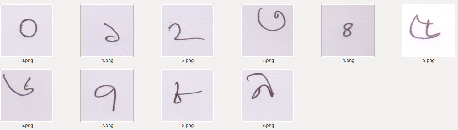
Fig 2: Bengali Handwritten Digits

At first, we'll load all the images to SparkData Frame. Then we build the model and train it. After that, we’ll evaluate the performance of our trained model.

Load Images

The data sets (from 0 to 9) contains almost 500 handwritten Bangla digits (50 images each class). Here, we manually load each image into a spark data-frame with a target column. After loading the whole dataset, we split into an 8:2 ratio randomly for the training set and final test set.

Our goal is to train the model with the training data set and finally evaluate the model’s performance with the test dataset.

# necessary import 
from pyspark.sql import SparkSession
from pyspark.ml.image import ImageSchema
from pyspark.sql.functions import lit
from functools import reduce

# create a spark session
spark = SparkSession.builder.appName(‘DigitRecog’).getOrCreate()

# loaded image
zero = ImageSchema.readImages("0").withColumn("label", lit(0))
one = ImageSchema.readImages("1").withColumn("label", lit(1))
two = ImageSchema.readImages("2").withColumn("label", lit(2))
three = ImageSchema.readImages("3").withColumn("label", lit(3))
four = ImageSchema.readImages("4").withColumn("label", lit(4))
five = ImageSchema.readImages("5").withColumn("label", lit(5))
six = ImageSchema.readImages("6").withColumn("label", lit(6))
seven = ImageSchema.readImages("7").withColumn("label", lit(7))
eight = ImageSchema.readImages("8").withColumn("label", lit(8))
nine = ImageSchema.readImages("9").withColumn("label", lit(9))

dataframes = [zero, one, two, three,four,
             five, six, seven, eight, nine]

# merge data frame
df = reduce(lambda first, second: first.union(second), dataframes)

# repartition dataframe 
df = df.repartition(200)

# split the data-frame
train, test = df.randomSplit([0.8, 0.2], 42)

Here, we can perform various Exploratory Data Analysis on Spark DataFrame. We can also view the schema of the data frame too.

df.printSchema()

root
 |-- image: struct (nullable = true)
 |    |-- origin: string (nullable = true)
 |    |-- height: integer (nullable = false)
 |    |-- width: integer (nullable = false)
 |    |-- nChannels: integer (nullable = false)
 |    |-- mode: integer (nullable = false)
 |    |-- data: binary (nullable = false)
 |-- label: integer (nullable = false)

We can also convert Spark-DataFrame to Pandas-DataFrame using .toPandas().

Model Training

Here, we combine the InceptionV3 model and logistic regression in the Spark node. The DeepImageFeaturizer automatically peels off the last layer of a pre-trained neural network and uses the output from all the previous layers as features for the logistic regression algorithm.

Since logistic regression is a simple and fast algorithm, this transfer learning training can converge quickly.

from pyspark.ml.evaluation import MulticlassClassificationEvaluator
from pyspark.ml.classification import LogisticRegression
from pyspark.ml import Pipeline
from sparkdl import DeepImageFeaturizer

# model: InceptionV3
# extracting feature from images
featurizer = DeepImageFeaturizer(inputCol="image",
                                 outputCol="features",
                                 modelName="InceptionV3")

# used as a multi class classifier
lr = LogisticRegression(maxIter=5, regParam=0.03, 
                        elasticNetParam=0.5, labelCol="label")

# define a pipeline model
sparkdn = Pipeline(stages=[featurizer, lr])
spark_model = sparkdn.fit(train) # start fitting or training

Evaluation

Now, it’s time to evaluate model performance. We now like to evaluate four evaluation metrics such as F1-score, Precision, Recall, Accuracy on the test data set.

from pyspark.ml.evaluation import MulticlassClassificationEvaluator

# evaluate the model with test set
evaluator = MulticlassClassificationEvaluator() 
tx_test = spark_model.transform(test)

print('F1-Score ', evaluator.evaluate(tx_test, 
                   {evaluator.metricName: 'f1'}))

print('Precision ', evaluator.evaluate(tx_test,
                   {evaluator.metricName: 'weightedPrecision'}))

print('Recall ', evaluator.evaluate(tx_test,   
                   {evaluator.metricName: 'weightedRecall'}))

print('Accuracy ', evaluator.evaluate(tx_test, 
                   {evaluator.metricName: 'accuracy'}))

Here we get the result. It’s promising until now.

F1-Score   0.8111782234361806
Precision  0.8422058244785519
Recall     0.8090909090909091
Accuracy   0.8090909090909091

Confusion Metrix

Here, we’ll summarize the performance of a classification model using the confusion matrix.

import matplotlib.pyplot as plt
import numpy as np
import itertools


def plot_confusion_matrix(cm, classes,
                          normalize=False,
                          title='Confusion matrix',
                          cmap=plt.cm.GnBu):

    plt.imshow(cm, interpolation='nearest', cmap=cmap)
    plt.title(title)
    tick_marks = np.arange(len(classes))
    plt.xticks(tick_marks, classes, rotation=45)
    plt.yticks(tick_marks, classes)

    fmt = '.2f' if normalize else 'd'
    thresh = cm.max() / 2.

    for i, j in itertools.product(range(cm.shape[0]), 
                                  range(cm.shape[1])):
        plt.text(j, i, format(cm[i, j], fmt),
                 horizontalalignment="center",
                 color="white" if cm[i, j] > thresh else "black")


    plt.tight_layout()
    plt.ylabel('True label')
    plt.xlabel('Predicted label')

For this, we need to convert Spark-DataFrame to Pandas-DataFrame first and then call Confusion Matrix with true and predicted labels.

from sklearn.metrics import confusion_matrix

y_true = tx_test.select("label")
y_true = y_true.toPandas()

y_pred = tx_test.select("prediction")
y_pred = y_pred.toPandas()

cnf_matrix = confusion_matrix(y_true, y_pred,labels=range(10))

Let’s visualize the Confusion Matrix

import seaborn as sns
sns.set_style("darkgrid")

plt.figure(figsize=(7,7))
plt.grid(False)

# call pre defined function
plot_confusion_matrix(cnf_matrix, classes=range(10))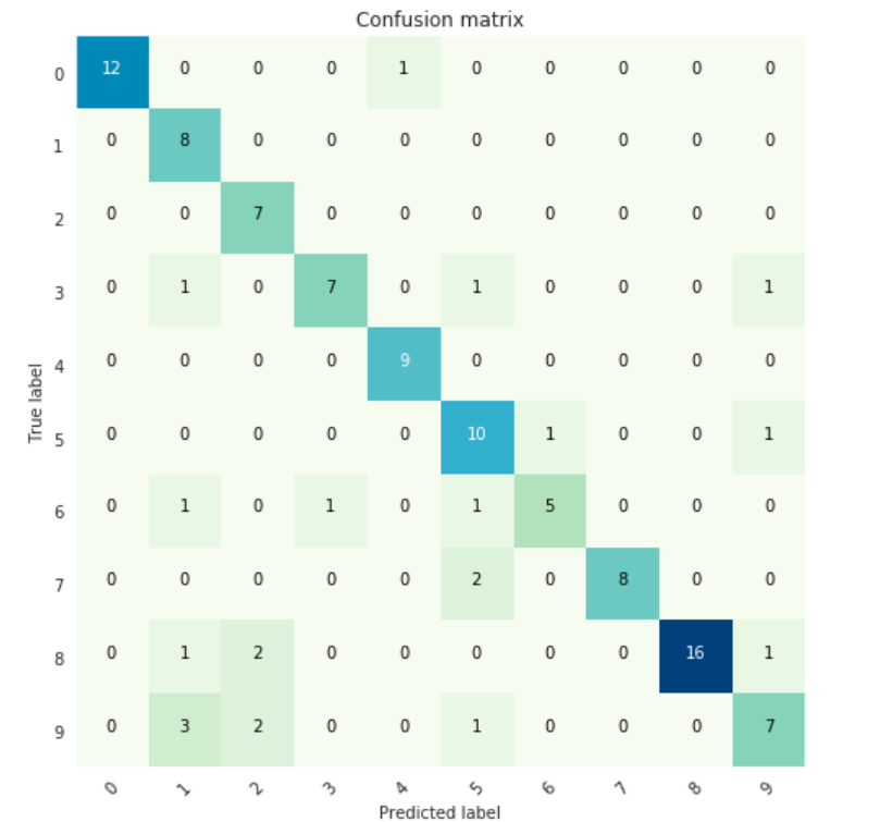

Fig 3: Confusion Matrix for 10 Bengali Digits (0 to 9)

Classification Report

Here, we can also get a report on the classification of each class by the evaluation matrix.

from sklearn.metrics import classification_report

target_names = ["Class {}".format(i) for i in range(10)]
print(classification_report(y_true, y_pred, 
                            target_names = target_names))

It’ll demonstrate much better the model performance for each class label prediction.

                 precision  recall   f1-score   support

     Class 0       1.00      0.92      0.96        13
     Class 1       0.57      1.00      0.73         8
     Class 2       0.64      1.00      0.78         7
     Class 3       0.88      0.70      0.78        10
     Class 4       0.90      1.00      0.95         9
     Class 5       0.67      0.83      0.74        12
     Class 6       0.83      0.62      0.71         8
     Class 7       1.00      0.80      0.89        10
     Class 8       1.00      0.80      0.89        20
     Class 9       0.70      0.54      0.61        13

   micro avg       0.81      0.81      0.81       110
   macro avg       0.82      0.82      0.80       110
weighted avg       0.84      0.81      0.81       110

ROC AUC Score

Let’s also find the ROC AUC score point of this model. I’ve used the following piece of code from here.

from sklearn.metrics import roc_curve, auc, roc_auc_score
from sklearn.preprocessing import LabelBinarizer

def multiclass_roc_auc_score(y_test, y_pred, average="macro"):
    lb = LabelBinarizer()
    lb.fit(y_test)
    y_test = lb.transform(y_test)
    y_pred = lb.transform(y_pred)
    return roc_auc_score(y_test, y_pred, average=average)

print('ROC AUC score:', multiclass_roc_auc_score(y_true,y_pred))

It scores 0.901.

Predicted Samples

Let’s see some of its prediction, comparison with the real label.

# all columns after transformations
print(tx_test.columns)

# see some predicted output
tx_test.select('image', "prediction", "label").show()

And the result would be as following

['image', 'label', 'features', 'rawPrediction', 
'probability', 'prediction']


+------------------+----------+--------+
|       image      |prediction|  label |
+------------------+----------+--------+
|[file:/home/i...|       1.0|    1|
|[file:/home/i...|       8.0|    8|
|[file:/home/i...|       9.0|    9|
|[file:/home/i...|       1.0|    8|
|[file:/home/i...|       1.0|    1|
|[file:/home/i...|       1.0|    9|
|[file:/home/i...|       0.0|    0|
|[file:/home/i...|       2.0|    9|
|[file:/home/i...|       8.0|    8|
|[file:/home/i...|       9.0|    9|
|[file:/home/i...|       0.0|    0|
|[file:/home/i...|       4.0|    0|
|[file:/home/i...|       5.0|    9|
|[file:/home/i...|       1.0|    1|
|[file:/home/i...|       9.0|    9|
|[file:/home/i...|       9.0|    9|
|[file:/home/i...|       1.0|    1|
|[file:/home/i...|       1.0|    1|
|[file:/home/i...|       9.0|    9|
|[file:/home/i...|       3.0|    6|
+--------------------+----------+-----+
only showing top 20 rows

Conclusion

Though we’ve used an ImageNet weight, our model performs pretty much promising to recognize handwritten digits. Moreover, we also didn’t perform any image processing tasks for better generalization. Also, the model is trained on very few amounts of data compared to the ImageNet dataset.

At a very high level, each Spark app consists of a driver program that launches various parallel operations on a cluster. The driver program contains our apps’ main function and defines distributed datasets on the cluster and then applies operations to them.

This is a standalone application where we’ve linked the application to Spark first and then we imported the Spark packages in our program and created a SparkContext initiated by a SparkSession. Though we’ve worked on a single machine, we can connect the same shell to a cluster to train data in parallel.

However, you can get the source code of today’s demonstration from here, and you can also follow me on GitHub for future code updates.

Next, we’ll look at Distributed Hyperparameter Tuning with Spark, and we'll try the custom Keras model and some new challenging examples.

References

Databricks: Deep Learning Guide
Apache Spark: PySpark Machine Learning