Using SingleStore DB, Spark and Alternating Least Squares (ALS) To Build a Movie Recommender System

Follow an example of building a movie recommender system to learn more about how to execute machine learning code directly in SingleStore DB.

Akmal Chaudhri

CORE ·

Mar. 24, 22 · Database Zone · Tutorial

Like (3)

Save

3.06K Views

Abstract

Recommender Systems are widely used today for many different applications. Examples include making product recommendations in e-commerce, restaurants, movies, music playlists, and more.

This article will show how to build a recommender system for movies using Alternating Least Squares (ALS). We'll perform some initial data analysis using Spark and then use its built-in support for ALS to generate vectors. We'll then store these vectors in SingleStore DB. Using SingleStore DB's built-in DOT_PRODUCT and UNHEX functions, we'll make movie recommendations by directly executing code in the database system.

The SQL scripts, Python code, and notebook files used in this article are available on GitHub. The notebook files are available in DBC, HTML, and iPython formats.

Introduction

An excellent article published in 2020 showed how to build a movie recommender system using Spark and MemSQL (MemSQL was the product name and company name before it became SingleStore). We can simplify the approach described in that article as follows:

We'll use Databricks Community Edition (CE) and SingleStore Cloud, thus keeping everything in the cloud.
We'll use Spark Dataframes without the need for any additional libraries, such as Pandas.
We'll use the SingleStore Spark Connector rather than SQLAlchemy.
We'll perform additional data analysis before loading any data into SingleStore DB.
We'll build a simple Streamlit application that allows us to see the movie recommendations, with movie posters, for a particular user.

To begin with, we need to create a free Cloud account on the SingleStore website, and a free Community Edition (CE) account on the Databricks website. At the time of writing, the Cloud account from SingleStore comes with $500 of Credits. This is more than adequate for the case study described in this article. For Databricks CE, we need to sign-up for the free account rather than the trial version. We are using Spark because, in a previous article, we noted that Spark was great for ETL with SingleStore DB.

We'll use the MovieLens 1m dataset. Before publishing this article, a form was completed, and permission was obtained to use the dataset. Further details about the MovieLens dataset can be found in the following article:

F. Maxwell Harper and Joseph A. Konstan. 2015. The MovieLens Datasets: History and Context. ACM Transactions on Interactive Intelligent Systems (TiiS) 5, 4, Article 19 (December 2015), 19 pages. DOI=http://dx.doi.org/10.1145/2827872

Once downloaded, we'll unpack the zip file from the dataset link above, which will give us a folder with four files:

movies.dat: Details of approximately 3900 movies
ratings.dat: Approximately 1 million movie ratings
users.dat: Details of approximately 6000 users
README: Important information about licensing and the structure of the three dat files.

We'll upload the three dat files to Databricks CE. Additionally, it would be great to have images of movie posters to render when building our Streamlit application. We can find a reference to a suitable dataset of movie poster hyperlinks in a discussion on GitHub, originally published under an MIT license. We'll use the movie_poster.csv file.

Configure Databricks CE

A previous article provides detailed instructions on how to Configure Databricks CE for use with SingleStore DB. We can use those exact instructions for this use case with several minor modifications. The modifications are that we will use:

Databricks Runtime version 9.1 LTS ML
The highest version of the SingleStore Spark Connector for Spark 3.1
The MariaDB Java Client 2.7.4 jar file

As shown in Figure 1, in addition to the SingleStore Spark Connector and the MariaDB Java Client jar file, we need to add WordCloud. This can be added using PyPI.

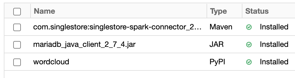
Figure 1. Libraries.

Upload DAT Files and CSV File

To use the DAT files and the CSV file, we need to upload them into the Databricks CE environment. A previous article provides detailed instructions on how to upload a CSV file. We can use those exact instructions for this use case.

Create Database Tables

In our SingleStore Cloud account, let's use the SQL Editor to create a new database. Call this recommender_db, as follows:

    SQL
   
   CREATE DATABASE IF NOT EXISTS recommender_db;

We'll also create the movies and users tables, as follows:

    SQL
   
 

   USE recommender_db;

CREATE TABLE movies (
     id INT PRIMARY KEY,
     title VARCHAR(255),
     genres VARCHAR(255),
     poster VARCHAR(255),
     factors BINARY(80)
);

CREATE TABLE users (
     id INT PRIMARY KEY,
     gender VARCHAR(5),
     age INT,
     occupation VARCHAR(255),
     zip_code VARCHAR(255),
     factors BINARY(80)
);
  

Fill Out the Notebook

Let's now create a new Databricks CE Python notebook. We'll call it Data Loader for Movie Recommender. We'll attach our new notebook to our Spark cluster.

Movies

Let's begin with movies. We'll first provide the movies schema, as follows:

    Python
   
   from pyspark.sql.types import *

separator = "::"

movies_schema = StructType([
  StructField("id", IntegerType(), True),
  StructField("title", StringType(), True),
  StructField("genres", StringType(), True)
])

Next, let's read the movies data into a Spark Dataframe:

    Python
   
 

   movies_df = spark.read.csv(
  "/FileStore/movies.dat",
  header = False,
  schema = movies_schema,
  sep = separator
)
  

In the following code cell, we'll take a look at the structure of the Dataframe:

    Python
   
   movies_df.show(5)

The output should be similar to this:

    Plain Text
   
 

   +---+--------------------+--------------------+
| id|               title|              genres|
+---+--------------------+--------------------+
|  1|    Toy Story (1995)|Animation|Childre...|
|  2|      Jumanji (1995)|Adventure|Childre...|
|  3|Grumpier Old Men ...|      Comedy|Romance|
|  4|Waiting to Exhale...|        Comedy|Drama|
|  5|Father of the Bri...|              Comedy|
+---+--------------------+--------------------+
only showing top 5 rows
  

We can generate a small word cloud, as follows:

    Python
   
 

   import matplotlib.pyplot as plt
from wordcloud import WordCloud, STOPWORDS, ImageColorGenerator

movie_titles = movies_df.select("title").collect()
movie_titles_list = [movie_titles[i][0] for i in range(len(movie_titles))]
movie_titles_corpus = (" ").join(title for title in movie_titles_list)

wordcloud = WordCloud(stopwords = STOPWORDS,
                      background_color = "lightgrey",
                      colormap = "hot",
                      max_words = 50,
                      # collocations = False,
                     ).generate(movie_titles_corpus)

plt.figure(figsize = (10, 8))
plt.imshow(wordcloud, interpolation = "bilinear")
plt.axis("off")
plt.show()
  

The result should be similar to Figure 2.

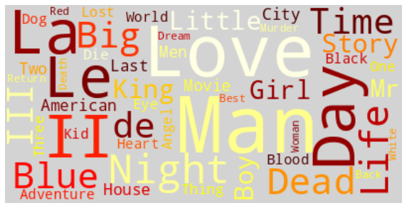
Figure 2. Word Cloud.

Perhaps no particular surprises in the word cloud.

We'll now create the schema for the movie posters, as follows:

    Python
   
   posters_schema = StructType([
  StructField("id", IntegerType(), True),
  StructField("poster", StringType(), True),
])

Create a new Dataframe, as follows:

    Python
   
 

   posters_df = spark.read.csv(
  "/FileStore/movie_poster.csv",
  header = False,
  schema = posters_schema
)
  

Next, we'll join the movies and posters Dataframes:

    Python
   
   movies_df = movies_df.join(
  posters_df,
  ["id"]
)

We can check the result as follows:

    Python
   
   movies_df.show(5)

The output should be similar to this:

    Plain Text
   
 

   +---+--------------------+--------------------+--------------------+
| id|               title|              genres|              poster|
+---+--------------------+--------------------+--------------------+
|  1|    Toy Story (1995)|Animation|Childre...|https://m.media-a...|
|  2|      Jumanji (1995)|Adventure|Childre...|https://m.media-a...|
|  3|Grumpier Old Men ...|      Comedy|Romance|https://m.media-a...|
|  4|Waiting to Exhale...|        Comedy|Drama|https://m.media-a...|
|  5|Father of the Bri...|              Comedy|https://m.media-a...|
+---+--------------------+--------------------+--------------------+
only showing top 5 rows
  

Users

Let's now turn to users. We'll first provide the users schema, as follows:

    Python
   
 

   users_schema = StructType([
  StructField("id", IntegerType(), True),
  StructField("gender", StringType(), True),
  StructField("age", IntegerType(), True),
  StructField("occupation_id", IntegerType(), True),
  StructField("zip_code", StringType(), True)
])
  

Next, let's read the users data into a Spark Dataframe:

    Python
   
 

   users_df = spark.read.csv(
  "/FileStore/users.dat",
  header = False,
  schema = users_schema,
  sep = separator
)
  

In the following code cell, we'll take a look at the structure of the Dataframe:

    Python
   
   users_df.show(5)

The output should be similar to this:

    Plain Text
   
 

   +---+------+---+-------------+--------+
| id|gender|age|occupation_id|zip_code|
+---+------+---+-------------+--------+
|  1|     F|  1|           10|   48067|
|  2|     M| 56|           16|   70072|
|  3|     M| 25|           15|   55117|
|  4|     M| 45|            7|   02460|
|  5|     M| 25|           20|   55455|
+---+------+---+-------------+--------+
only showing top 5 rows
  

Let's now perform a quick analysis of gender, as follows:

    Python
   
 

   (users_df
  .groupBy("gender")
  .count()
  .show()
)
  

The output shows that the users are approximately 70% male and 30% female:

    Plain Text
   
 

   +------+-----+
|gender|count|
+------+-----+
|     F| 1709|
|     M| 4331|
+------+-----+
  

Occupation is stored as a numeric value, but the mapping is described in the README file. We can create a list and schema as follows:

    Python
   
 

   occupations = [( 0, "other"),
               ( 1, "academic/educator"),
               ( 2, "artist"),
               ( 3, "clerical/admin"),
               ( 4, "college/grad student"),
               ( 5, "customer service"),
               ( 6, "doctor/health care"),
               ( 7, "executive/managerial"),
               ( 8, "farmer"),
               ( 9, "homemaker"),
               (10, "K-12 student"),
               (11, "lawyer"),
               (12, "programmer"),
               (13, "retired"),
               (14, "sales/marketing"),
               (15, "scientist"),
               (16, "self-employed"),
               (17, "technician/engineer"),
               (18, "tradesman/craftsman"),
               (19, "unemployed"),
               (20, "writer")]

occupations_schema = StructType([
  StructField("occupation_id", IntegerType(), True),
  StructField("occupation", StringType(), True)
])
  

Using this information, we can create a new Dataframe, as follows:

    Python
   
   occupations_df = spark.createDataFrame(
  data = occupations,
  schema = occupations_schema
)

We can now join the users and occupations Dataframes so that we can get the correct occupation description and then drop any columns that we don't need, as follows:

    Python
   
 

   users_df = users_df.join(
  occupations_df,
  ["occupation_id"]
)

users_df = users_df.drop(
  "occupation_id"
)
  

Now, we'll check the structure of the users Dataframe:

    Python
   
   users_df.show(5)

The output should be similar to this:

    Plain Text
   
 

   +----+------+---+--------+----------+
|  id|gender|age|zip_code|occupation|
+----+------+---+--------+----------+
|6039|     F| 45|   01060|     other|
|6031|     F| 18|   45123|     other|
|6023|     M| 25|   43213|     other|
|6019|     M| 25|   10024|     other|
|6010|     M| 35|   79606|     other|
+----+------+---+--------+----------+
only showing top 5 rows
  

We can also analyze the distribution of occupations, as follows:

    Python
   
 

   (users_df
  .groupBy("occupation")
  .count()
  .orderBy("count", ascending = False)
  .show(21)
)
  

The output should be similar to this:

    Plain Text
   
 

   +--------------------+-----+
|          occupation|count|
+--------------------+-----+
|college/grad student|  759|
|               other|  711|
|executive/managerial|  679|
|   academic/educator|  528|
| technician/engineer|  502|
|          programmer|  388|
|     sales/marketing|  302|
|              writer|  281|
|              artist|  267|
|       self-employed|  241|
|  doctor/health care|  236|
|        K-12 student|  195|
|      clerical/admin|  173|
|           scientist|  144|
|             retired|  142|
|              lawyer|  129|
|    customer service|  112|
|           homemaker|   92|
|          unemployed|   72|
| tradesman/craftsman|   70|
|              farmer|   17|
+--------------------+-----+
  

Ratings

Next, let's focus on ratings. We'll first provide the ratings schema, as follows:

    Python
   
 

   ratings_schema = StructType([
  StructField("user_id", IntegerType(), True),
  StructField("movie_id", IntegerType(), True),
  StructField("rating", IntegerType(), True),
  StructField("timestamp", IntegerType(), True)
])
  

Next, let's read the ratings data into a Spark Dataframe:

    Python
   
 

   ratings_df = spark.read.csv(
  "/FileStore/ratings.dat",
  header = False,
  schema = ratings_schema,
  sep = separator
)
  

In the following code cell, we'll take a look at the structure of the DataFrame:

    Python
   
   ratings_df.show(5)

The output should be similar to this:

    Plain Text
   
 

   +-------+--------+------+---------+
|user_id|movie_id|rating|timestamp|
+-------+--------+------+---------+
|      1|    1193|     5|978300760|
|      1|     661|     3|978302109|
|      1|     914|     3|978301968|
|      1|    3408|     4|978300275|
|      1|    2355|     5|978824291|
+-------+--------+------+---------+
only showing top 5 rows
  

We can get some additional information, as follows:

    Python
   
   (ratings_df
  .describe("user_id", "movie_id", "rating")
  .show()
)

The output should be similar to this:

    Plain Text
   
 

   +-------+------------------+------------------+------------------+
|summary|           user_id|          movie_id|            rating|
+-------+------------------+------------------+------------------+
|  count|           1000209|           1000209|           1000209|
|   mean| 3024.512347919285|1865.5398981612843| 3.581564453029317|
| stddev|1728.4126948999715|1096.0406894572482|1.1171018453732606|
|    min|                 1|                 1|                 1|
|    max|              6040|              3952|                 5|
+-------+------------------+------------------+------------------+
  

We can see that the average movie rating appears quite generous.

We can generate a small rating histogram, as follows:

    Python
   
 

   movie_ratings = ratings_df.select("rating").collect()
movie_ratings_list = [movie_ratings[i][0] for i in range(len(movie_ratings))]

plt.hist(
  movie_ratings_list,
  edgecolor = "white",
  color = "#32B5C9",
  rwidth = 0.9,
  bins = [0.5, 1.5, 2.5, 3.5, 4.5, 5.5]
)

plt.ylabel("Frequency")
plt.xlabel("Rating")
plt.show()
  

The result should be similar to Figure 3.

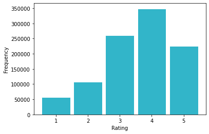
Figure 3. Rating Histogram.

Alternating Least Squares (ALS)

Let's start by creating our train and test sets, as follows:

    Python
   
   (train, test) = ratings_df.randomSplit([0.7, 0.3], seed = 123)

We'll now use Spark's ALS implementation to create our model:

    Python
   
 

   from pyspark.ml.recommendation import ALS

als = ALS(
  maxIter = 5,
  regParam = 0.01,
  userCol = "user_id",
  itemCol = "movie_id",
  ratingCol = "rating",
  coldStartStrategy = "drop",
  seed = 0
)

model = als.fit(train)
  

We can then show the predictions on the test data, as follows:

    Python
   
   from pyspark.ml.evaluation import RegressionEvaluator

predictions = model.transform(test)

predictions.show(5)

The output should be similar to this:

    Plain Text
   
 

   +-------+--------+------+---------+----------+
|user_id|movie_id|rating|timestamp|prediction|
+-------+--------+------+---------+----------+
|    148|       1|     5|977335193| 4.3501983|
|    148|       2|     5|979578366| 3.8232095|
|    148|      11|     5|977334939|  4.321706|
|    148|      50|     2|979577217| 3.8569245|
|    148|      60|     3|979578136| 3.6407182|
+-------+--------+------+---------+----------+
only showing top 5 rows
  

We can determine the RMSE as follows:

    Python
   
 

   re = RegressionEvaluator(
  predictionCol = "prediction",
  labelCol = "rating",
  metricName = "rmse"
)

rmse = re.evaluate(predictions)
print(rmse)
  

The result should be similar to this:

    Plain Text
   
   0.9147891485260777

We can view the user factors as follows:

    Python
   
   model.userFactors.show(5) # show(5, False) to show the whole column

The output should be similar to this:

    Plain Text
   
 

   +---+--------------------+
| id|            features|
+---+--------------------+
| 10|[0.8803474, 0.799...|
| 20|[0.47382107, 0.65...|
| 30|[0.8101255, -0.38...|
| 40|[-0.008799124, 0....|
| 50|[-0.33016467, 0.4...|
+---+--------------------+
only showing top 5 rows
  

For example, the first line (id = 10) would be as follows:

    Plain Text
   
   [0.8803474, 0.7996457, -1.3396101, 1.8472301, 0.7709434, 1.4858658, 0.5260316, 1.5704685, 0.14094345, 0.022391517]

Similarly, we can view the item (movie) factors as follows:

    Python
   
   model.itemFactors.show(5) # show(5, False) to show the whole column

The output should be similar to this:

    Plain Text
   
 

   +---+--------------------+
| id|            features|
+---+--------------------+
| 10|[0.08083672, 0.60...|
| 20|[0.5918954, 0.415...|
| 30|[-0.047557604, -0...|
| 40|[-1.0247108, 1.19...|
| 50|[0.1312179, -0.08...|
+---+--------------------+
only showing top 5 rows
  

For example, the first line (id = 10) would be as follows:

    Plain Text
   
   [0.08083672, 0.60175675, -0.34102643, 0.4448118, 0.81003183, 0.50796205, 0.5284808, 0.009832226, 0.2445135, 0.1576684]

Now that we have these two different vectors, we can store them in SingleStore DB. However, to do this, we need to convert them to a format that SingleStore DB understands. The SingleStore DB documentation provides guidance on acceptable vector formats.

First, let's create two Dataframes, as follows:

    Python
   
   user_factors_df = model.userFactors
item_factors_df = model.itemFactors

Next, let's create and register a UDF with Spark that will perform the data conversion for us:

    Python
   
 

   import array, binascii

def vector_to_hex(vector):
  vector_bytes = bytes(array.array("f", vector))
  vector_hex = binascii.hexlify(vector_bytes)
  vector_string = str(vector_hex.decode())
  return vector_string

vector_to_hex = udf(vector_to_hex, StringType())
spark.udf.register("vector_to_hex", vector_to_hex)
  

Let's see how this UDF works with an example. Let's take some data from earlier:

    Python
   
   vector = [0.8803474, 0.7996457, -1.3396101, 1.8472301, 0.7709434, 1.4858658, 0.5260316, 1.5704685, 0.14094345, 0.022391517]

Using the following line:

    Python
   
   vector_bytes = bytes(array.array("f", vector))

We will convert our above vector to the following representation:

    Plain Text
   
   b'r^a?\x95\xb5L?Xx\xab\xbf\tr\xec?\x8c\\E?\xda0\xbe?\x02\xaa\x06?\x1d\x05\xc9?{S\x10>jn\xb7<'

The next line:

    Python
   
   vector_hex = binascii.hexlify(vector_bytes)

Will then convert the previous output to the following representation:

    Plain Text
   
   b'725e613f95b54c3f5878abbf0972ec3f8c5c453fda30be3f02aa063f1d05c93f7b53103e6a6eb73c'

Finally, the following line:

    Python
   
   vector_string = str(vector_hex.decode())

Will give us the data in the format that we can store in SingleStore DB:

    Plain Text
   
   725e613f95b54c3f5878abbf0972ec3f8c5c453fda30be3f02aa063f1d05c93f7b53103e6a6eb73c

We can now apply the UDF to the two Dataframes, as follows:

    Python
   
 

   user_factors_df = user_factors_df.withColumn(
  "factors",
  vector_to_hex("features")
)

item_factors_df = item_factors_df.withColumn(
  "factors",
  vector_to_hex("features")
)
  

We can now join the users and movies Dataframes with their respective factors Dataframes and then drop any columns that we don't need. First, users:

    Python
   
   users = users_df.join(
  user_factors_df,
  ["id"]
)

users = users.drop("features")

Next, movies:

    Python
   
   movies = movies_df.join(
  item_factors_df,
  ["id"]
)

movies = movies.drop("features")

Write Data To SingleStore DB

We are now ready to write the users and movies Dataframes to SingleStore DB. In the following code cell, we can add the following:

    Python
   
   %run ./Setup

In the Setup notebook, we need to ensure that the server address and password have been added for our SingleStore Cloud cluster.

In the following code cell, we'll set some parameters for the SingleStore Spark Connector, as follows:

    Python
   
   spark.conf.set("spark.datasource.singlestore.ddlEndpoint", cluster)
spark.conf.set("spark.datasource.singlestore.user", "admin")
spark.conf.set("spark.datasource.singlestore.password", password)
spark.conf.set("spark.datasource.singlestore.disablePushdown", "false")

Finally, we are ready to write the Dataframes to SingleStore DB using the Spark Connector. First, users:

    Python
   
 

   (users.write
   .format("singlestore")
   .option("loadDataCompression", "LZ4")
   .mode("ignore")
   .save("recommender_db.users")
)
  

Next, movies:

    Python
   
 

   (movies.write
   .format("singlestore")
   .option("loadDataCompression", "LZ4")
   .mode("ignore")
   .save("recommender_db.movies")
)
  

We can check that the two database tables were successfully populated from SingleStore Cloud.

Example Queries

Now that we have built our system, we can run some queries. Let's include the three example queries from the article referenced earlier.

First, let's make movie recommendations for the user with id = 1, as follows:

    SQL
   
 

   SELECT movies.title,
       movies.genres,
       DOT_PRODUCT(UNHEX(users.factors), UNHEX(movies.factors)) AS score
FROM users JOIN movies
WHERE users.id = 1
ORDER BY score DESC
LIMIT 10;
  

This produces the following output shown in Figure 4:

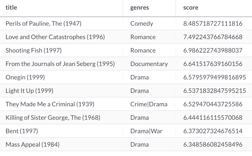
Figure 4. Movie Recommendations.

We can also make user recommendations for the movie with id = 1, as follows:

    SQL
   
 

   SELECT users.gender,
       users.age,
       users.occupation,
       users.zip_code,
       DOT_PRODUCT(UNHEX(movies.factors), UNHEX(users.factors)) AS score
FROM movies JOIN users
WHERE movies.id = 1
ORDER BY score DESC
LIMIT 10;
  

This produces the following output shown in Figure 5:

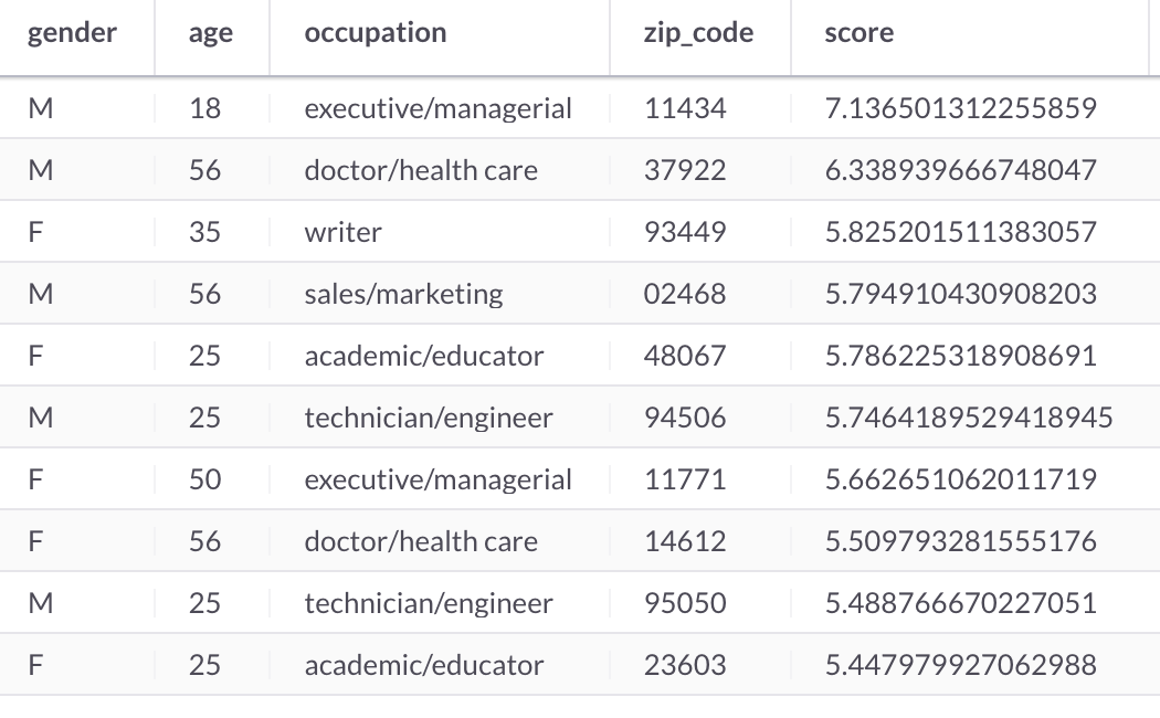
Figure 5. User Recommendations.

Next, let's make Sci-Fi movie recommendations for the 1980s for the same user, as follows:

    SQL
   
 

   SELECT movies.title,
       movies.genres,
       DOT_PRODUCT(UNHEX(users.factors), UNHEX(movies.factors)) AS score
FROM users JOIN movies
WHERE users.id = 1 AND
       SUBSTRING(movies.title, -3, 1) = 8 AND
       movies.genres LIKE '%sci-fi%'
ORDER BY score DESC
LIMIT 10;
  

This produces the following output shown in Figure 6:

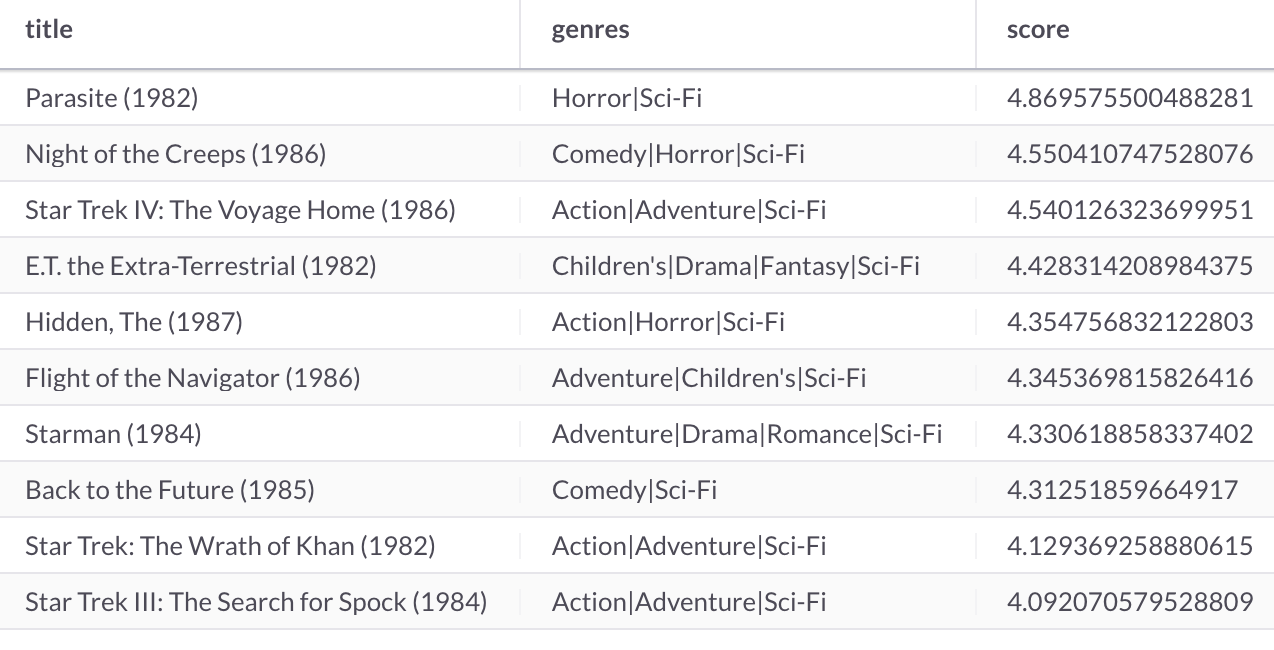
Figure 6. Movie Recommendations.

Finally, let's make movie recommendations for a new Male user that is within the 18-24 age range, as follows:

    SQL
   
 

   SELECT movies.title,
       movies.genres,
       AVG(DOT_PRODUCT(UNHEX(users.factors), UNHEX(movies.factors))) AS avg_score,
       count(1) AS c
FROM users JOIN movies
WHERE users.gender = 'M' AND
       users.age = 18 AND
       DOT_PRODUCT(UNHEX(users.factors), UNHEX(movies.factors)) > 5
GROUP BY 1, 2
ORDER BY avg_score DESC
LIMIT 10;
  

This produces the following output shown in Figure 7:

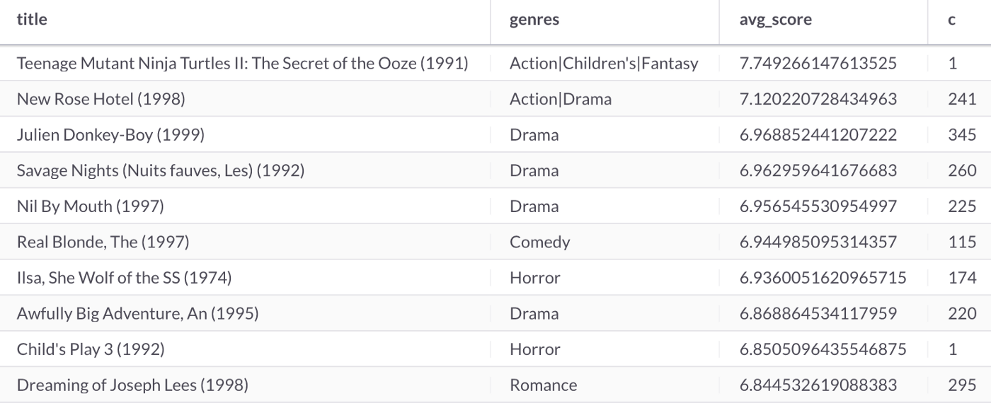
Figure 7. Movie Recommendations.

Bonus: Streamlit Visualization

We can build a small application for the first query above and render images for movie posters. We can do this quite easily with Streamlit. A previous article showed the ease with which we could connect Streamlit to SingleStore DB.

Install the Required Software

We need to install the following packages:

    Plain Text
   
   streamlit
pandas
pymysql

These can be found in the requirements.txt file on GitHub. Run the file as follows:

    Shell
   
   pip install -r requirements.txt

Example Application

Here is the complete code listing for streamlit_app.py:

    Python
   
 

   # streamlit_app.py
import streamlit as st
import pandas as pd
import pymysql

# Initialize connection.

def init_connection():
    return pymysql.connect(**st.secrets["singlestore"])

conn = init_connection()

user_id = st.sidebar.number_input("Enter a User Id", min_value = 1, max_value = 6040)

# Perform query.

data = pd.read_sql("""
SELECT movies.title,
       movies.poster,
       DOT_PRODUCT(UNHEX(users.factors), UNHEX(movies.factors)) AS score
FROM users JOIN movies
WHERE users.id = %s
ORDER BY score DESC
LIMIT 10;
""", conn, params = ([str(user_id)]))

st.subheader("Movie Recommendations")

for i in range(10):
   cols = st.columns(1)
   cols[0].header(data["title"][i])
   cols[0].image(data["poster"][i], width = 200)
  

Create a Secrets File

Our local Streamlit application will read secrets from a file .streamlit/secrets.toml in our application's root directory. We need to create this file as follows:

    Plain Text
   
 

   # .streamlit/secrets.toml

[singlestore]
host = "<TO DO>"
port = 3306
database = "recommender_db"
user = "admin"
password = "<TO DO>"
  

The <TO DO> for host and password should be replaced with the values obtained from SingleStore Cloud when creating a cluster.

Run the Code

We can run the Streamlit application as follows:

    Shell
   
   streamlit run streamlit_app.py

The output in a web browser should look like Figure 8.

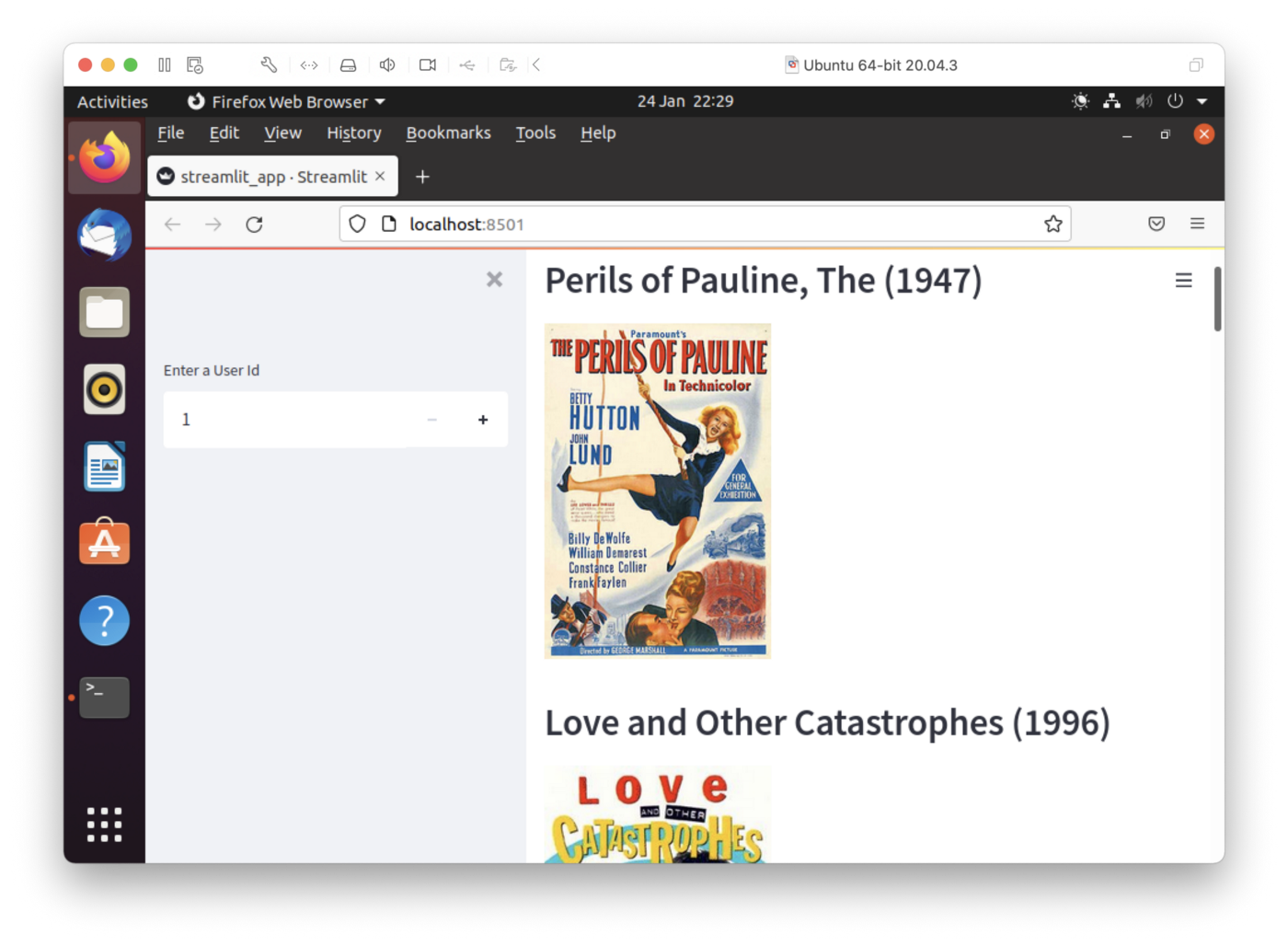
Figure 8. Streamlit.

We can enter a new user id in the input box on the left-hand side of the web page. The top 10 movie recommendations are shown on the right-hand side. Feel free to experiment with the code to suit your needs.

Summary

This article has built a movie recommender system using SingleStore DB, Spark, and Alternating Least Squares. We have seen how we can store vectors in SingleStore DB and using the built-in functions, DOT_PRODUCT and UNHEX, we can perform operations on those vectors directly in the database system. We can make movie recommendations for existing users and predictions for new users using these built-in functions.

Published at DZone with permission of Akmal Chaudhri. See the original article here.

Opinions expressed by DZone contributors are their own.

Comments

Using SingleStore DB, Spark and Alternating Least Squares (ALS) To Build a Movie Recommender System

Follow an example of building a movie recommender system to learn more about how to execute machine learning code directly in SingleStore DB.

Abstract

Introduction

Configure Databricks CE

Upload DAT Files and CSV File

Create Database Tables

Fill Out the Notebook

Movies

Users

Ratings

Alternating Least Squares (ALS)

Write Data To SingleStore DB

Example Queries

Bonus: Streamlit Visualization

Install the Required Software

Example Application

Create a Secrets File

Run the Code

Summary

Popular on DZone

Database Partner Resources