ANSI JOIN Support in N1QL

ANSI JOIN support was added in N1QL to Couchbase version 5.5. Previous versions of Couchbase only support lookup joins and index joins. Lookup joins and index joins work great when the document key from one side of the join can be produced by the other side of the join, i.e. joining on a parent-child or child-parent relationship through a document key. Where they fall short is when the join is on arbitrary fields or expressions of fields or when multiple join conditions are required. ANSI JOIN is a standardized join syntax widely used in relational databases. ANSI JOIN is much more flexible than lookup joins and index joins, allowing joins to be done on arbitrary expressions on any fields in a document. This makes join operations much simpler and more powerful.

ANSI JOIN syntax:

lhs-expression [ join-type ] JOIN rhs-keyspace ON [ join-condition ]

The left-hand side of the join, lhs-expression, can be a keyspace, an N1QL expression, a subquery, or a previous join. The right-hand side of the join, rhs-keyspace, must be a keyspace. The ON clause specifies the join-condition, which can be any arbitrary expression, although it should contain predicates that allow an index scan on the right-hand side keyspace. join-type can be INNER, LEFT OUTER, or RIGHT OUTER. The INNER and OUTER keywords are optional, so JOIN is the same as INNER JOIN and LEFT JOIN is the same as LEFT OUTER JOIN. In relational databases, join-type can also be FULL OUTER or CROSS, although FULL OUTER JOIN and CROSS JOIN are not supported currently in N1QL.

Details of ANSI JOIN Support

We’ll use examples to show you new ways you can run queries using ANSI JOIN syntax and how to transform your existing join queries in N1QL from lookup join or index join syntax into new ANSI JOIN syntax. It should be noted that lookup joins and index joins will continue to be supported in N1QL for backward compatibility; however, you cannot mix lookup joins or index joins with the new ANSI JOIN syntax in the same query block, so customers are encouraged to migrate to the new ANSI JOIN syntax.

To follow along, install this travel-sample sample bucket.

Example 1: ANSI JOIN With Arbitrary Join-Condition

join-condition (ON clause) for ANSI JOIN can be any expression involving any fields of the documents being joined. For example...

Required index:

CREATE INDEX route_airports ON `travel-sample`(sourceairport, destinationairport) WHERE type = "route";

Optional index:

CREATE INDEX airport_city_country ON `travel-sample`(city, country) WHERE type = "airport";

Query:

SELECT DISTINCT route.destinationairport
FROM `travel-sample` airport JOIN `travel-sample` route
     ON airport.faa = route.sourceairport
        AND route.type = "route"
WHERE airport.type = "airport"
  AND airport.city = "San Francisco"
  AND airport.country = "United States";

In this query, we are joining a field (faa) from the airport document with a field (sourceairport) from the route document (see the ON clause of the join). Such a join is not possible with a lookup join or index join in N1QL since both require joining on a document key only.

ANSI JOIN requires an appropriate index on the right-hand side keyspace (“Required index” above). You can also create other indexes (“Optional index” above) to speed up your query. Without the optional index, a primary scan will be used and the query still works; however, without the required index, the query will not work and will return an error.

Looking at the explain:

"plan": {
   "#operator": "Sequence",
   "~children": [
       {
           "#operator": "IndexScan3",
           "as": "airport",
           "index": "airport_city_country",
           "index_id": "8e782fd1b124eec3",
           "index_projection": {
               "primary_key": true
           },
           "keyspace": "travel-sample",
           "namespace": "default",
           "spans": [
               {
                   "exact": true,
                   "range": [
                       {
                           "high": "\"San Francisco\"",
                           "inclusion": 3,
                           "low": "\"San Francisco\""
                       },
                       {
                           "high": "\"United States\"",
                           "inclusion": 3,
                           "low": "\"United States\""
                       }
                   ]
               }
           ],
           "using": "gsi"
       },
       {
           "#operator": "Fetch",
           "as": "airport",
           "keyspace": "travel-sample",
           "namespace": "default"
       },
       {
           "#operator": "Parallel",
           "~child": {
               "#operator": "Sequence",
               "~children": [
                   {
                       "#operator": "NestedLoopJoin",
                       "alias": "route",
                       "on_clause": "(((`airport`.`faa`) = cover ((`route`.`sourceairport`))) and (cover ((`route`.`type`)) = \"route\"))",
                       "~child": {
                           "#operator": "Sequence",
                           "~children": [
                               {
                                   "#operator": "IndexScan3",
                                   "as": "route",
                                   "covers": [
                                       "cover ((`route`.`sourceairport`))",
                                       "cover ((`route`.`destinationairport`))",
                                       "cover ((meta(`route`).`id`))"
                                   ],
                                   "filter_covers": {
                                       "cover ((`route`.`type`))": "route"
                                   },
                                   "index": "route_airports",
                                   "index_id": "f1f4b9fbe85e45fd",
                                   "keyspace": "travel-sample",
                                   "namespace": "default",
                                   "nested_loop": true,
                                   "spans": [
                                       {
                                           "exact": true,
                                           "range": [
                                               {
                                                   "high": "(`airport`.`faa`)",
                                                   "inclusion": 3,
                                                   "low": "(`airport`.`faa`)"
                                               }
                                           ]
                                       }
                                   ],
                                   "using": "gsi"
                               }
                           ]
                       }
                   },
                   {
                       "#operator": "Filter",
                       "condition": "((((`airport`.`type`) = \"airport\") and ((`airport`.`city`) = \"San Francisco\")) and ((`airport`.`country`) = \"United States\"))"
                   },
                   {
                       "#operator": "InitialProject",
                       "distinct": true,
                       "result_terms": [
                           {
                               "expr": "cover ((`route`.`destinationairport`))"
                           }
                       ]
                   },
                   {
                       "#operator": "Distinct"
                   },
                   {
                       "#operator": "FinalProject"
                   }
               ]
           }
       },
       {
           "#operator": "Distinct"
       }
   ]
}

You will see that a NestedLoopJoin operator is used to perform the join, and underneath that, an IndexScan3 operator is used to access the right-hand side keyspace, route. The spans for the index scan look like:

"spans": [
   {
       "exact": true,
       "range": [
           {
               "high": "(`airport`.`faa`)",
               "inclusion": 3,
               "low": "(`airport`.`faa`)"
           }
       ]
   }
]

The index scan for the right-hand side keyspace (route) is using a field (faa) from the left-hand side keyspace (airport) as a search key. For each document from the outer side keyspace airport, the NestedLoopJoin operator performs an index scan on the inner side keyspace route to find matching documents and produces join results. The join is performed in a nested-loop fashion, where the outer loop produces a document from the outer side keyspace and a nested inner loop searches for a matching inner side document for the current outer side document.

The explain information can also be viewed graphically on Query Workbench by clicking the Explain button followed by the Plan button:

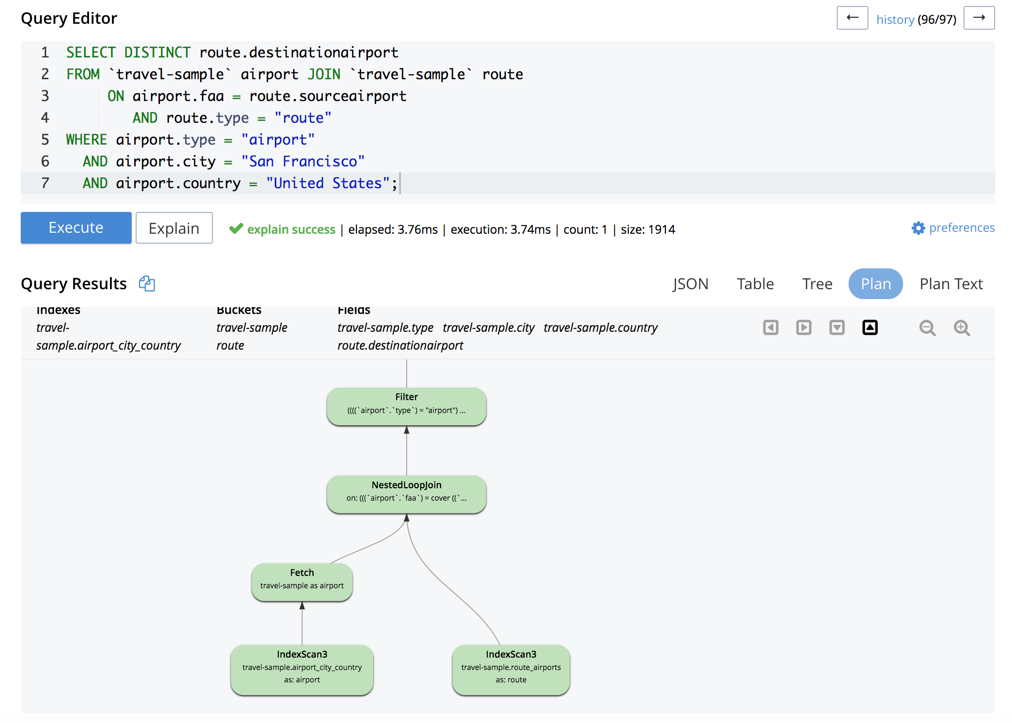
In this example, the index scan on the right-hand side keyspace is a covered index scan. In case the index scan is not covered, a fetch operator will be following the index scan operator to fetch the document.

It should be noted that a nested-loop join requires an appropriate secondary index on the right-hand side keyspace of an ANSI JOIN. The primary index is not considered for this purpose. If an appropriate secondary cannot be found, an error will be returned for the query.

In addition, you might have noticed that the filter route.type = "route" appears in the ON clause, as well. The ON clause is different than the WHERE clause in that the ON clause is evaluated as part of the join, while the WHERE clause is evaluated after all joins are done. This distinction is important, especially for outer joins. Therefore, it is recommended that you include filters on the right-hand side keyspace for a join in the ON clause as well, in addition to any join filters.

Example 2: ANSI JOIN With Multiple Join-Conditions

While lookup joins and index joins only join on a single join-conditions (equality of document key), the ON clause of an ANSI JOIN can contain multiple join-conditions.

Required index:

CREATE INDEX landmark_city_country ON `travel-sample`(city, country) WHERE type = "landmark";

Optional index:

CREATE INDEX hotel_title ON `travel-sample`(title) WHERE type = "hotel";

Query:

SELECT hotel.name hotel_name, landmark.name landmark_name, landmark.activity
FROM `travel-sample` hotel JOIN `travel-sample` landmark
    ON hotel.city = landmark.city AND hotel.country = landmark.country AND landmark.type = "landmark"
WHERE hotel.type = "hotel" AND hotel.title like "Yosemite%" AND array_length(hotel.public_likes) > 5;

Looking at the explain, the index spans for the index (landmark_city_country) of the right-hand side keyspace (landmark) is:

"spans": [
   {
       "exact": true,
       "range": [
           {
               "high": "(`hotel`.`city`)",
               "inclusion": 3,
               "low": "(`hotel`.`city`)"
           },
           {
               "high": "(`hotel`.`country`)",
               "inclusion": 3,
               "low": "(`hotel`.`country`)"
           }
       ]
   }
]

Thus, multiple join predicates can potentially generate multiple index search keys for the index scan of the inner side of a nested-loop join.

Example 3: ANSI JOIN With Complex Join Expressions

The join-condition in the ON clause can be a complex join expression. For example, the airlineid field in the route document corresponds to the document key for the airline document, but it can also be constructed by concatenating airline_ with the id field of the airline document.

Required index:

CREATE INDEX route_airlineid ON `travel-sample`(airlineid) WHERE type = "route";

Optional index:

CREATE INDEX airline_name ON `travel-sample`(name) WHERE type = "airline";

Query:

SELECT count(*)
FROM `travel-sample` airline JOIN `travel-sample` route
     ON route.airlineid = "airline_" || tostring(airline.id) AND route.type = "route"
WHERE airline.type = "airline" AND airline.name = "United Airlines";

The explain contains the following index spans for the right-hand side keyspace (route):

"spans": [
   {
       "exact": true,
       "range": [
           {
               "high": "(\"airline_\" || to_string((`airline`.`id`)))",
               "inclusion": 3,
               "low": "(\"airline_\" || to_string((`airline`.`id`)))"
           }
       ]
   }
]

The expression will be evaluated at runtime to generate the search keys for the index scan on the inner side of the nested-loop join.

Example 4: ANSI JOIN With IN Clause

join-condition does not need to be an equality predicate. An IN clause can be used as join-condition.

Required index:

CREATE INDEX airport_faa_name ON `travel-sample`(faa, airportname) WHERE type = "airport";

Optional index:

CREATE INDEX route_airline_distance ON `travel-sample`(airline, distance) WHERE type = "route";

Query:

SELECT DISTINCT airport.airportname
FROM `travel-sample` route JOIN `travel-sample` airport
    ON airport.faa IN [ route.sourceairport, route.destinationairport ] AND airport.type = "airport"
WHERE route.type = "route" AND route.airline = "F9" AND route.distance > 3000;

The explain contains the following index spans for the right-hand side keyspace (airport):

"spans": [
    {
        "range": [
            {
                "high": "(`route`.`sourceairport`)",
                "inclusion": 3,
                "low": "(`route`.`sourceairport`)"
            }
        ]
    },
    {
        "range": [
            {
                "high": "(`route`.`destinationairport`)",
                "inclusion": 3,
                "low": "(`route`.`destinationairport`)"
            }
        ]
    }
]

Example 5: ANSI JOIN With OR Clause

Similar to the IN clause, join-condition for an ANSI JOIN can also contain an OR clause. Different arms of the OR clause can potentially reference different fields of the right-hand side keyspace, as long as appropriate indexes exist.

Required index (route_airports index, same as Example 1):

CREATE INDEX route_airports ON `travel-sample`(sourceairport, destinationairport) WHERE type = "route";
CREATE INDEX route_airports2 ON `travel-sample`(destinationairport, sourceairport) WHERE type = "route";

Optional index (same as Example 1):

CREATE INDEX airport_city_country ON `travel-sample`(city, country) WHERE type = "airport";

Query:

SELECT count(*)
FROM `travel-sample` airport JOIN `travel-sample` route
    ON (route.sourceairport = airport.faa OR route.destinationairport = airport.faa) AND route.type = "route"
WHERE airport.type = "airport" AND airport.city = "Denver" AND airport.country = "United States";

The explain shows an UnionScan being used under NestedLoopJoin to handle the OR clause:

"#operator": "UnionScan",
"scans": [
   {
       "#operator": "IndexScan3",
       "as": "route",
       "index": "route_airports",
       "index_id": "f1f4b9fbe85e45fd",
       "index_projection": {
           "primary_key": true
       },
       "keyspace": "travel-sample",
       "namespace": "default",
       "nested_loop": true,
       "spans": [
           {
               "exact": true,
               "range": [
                   {
                       "high": "(`airport`.`faa`)",
                       "inclusion": 3,
                       "low": "(`airport`.`faa`)"
                   }
               ]
           }
       ],
       "using": "gsi"
   },
   {
       "#operator": "IndexScan3",
       "as": "route",
       "index": "route_airports2",
       "index_id": "cdc9dca18c973bd3",
       "index_projection": {
           "primary_key": true
       },
       "keyspace": "travel-sample",
       "namespace": "default",
       "nested_loop": true,
       "spans": [
           {
               "exact": true,
               "range": [
                   {
                       "high": "(`airport`.`faa`)",
                       "inclusion": 3,
                       "low": "(`airport`.`faa`)"
                   }
               ]
           }
       ],
       "using": "gsi"
   }
]

Example 6: ANSI JOIN With Hints

For lookup joins and index joins, hints can only be specified on the keyspace on the left-hand side of the join. For ANSI JOINs, hints can be specified on the right-hand side keyspace, as well. Using the same query as Example 1 (with the addition of the USE INDEX hint)...

SELECT DISTINCT route.destinationairport
FROM `travel-sample` airport JOIN `travel-sample` route USE INDEX(route_airports)
    ON airport.faa = route.sourceairport AND route.type = "route"
WHERE airport.type = "airport" AND airport.city = "San Francisco" AND airport.country = "United States";

The USE INDEX hint limits the number of indexes the planner needs to consider for performing the join.

Hints can also be specified on the left-hand side keyspace of ANSI JOIN.

SELECT DISTINCT route.destinationairport
FROM `travel-sample` airport USE INDEX(airport_city_country)
  JOIN `travel-sample` route USE INDEX(route_airports)
    ON airport.faa = route.sourceairport AND route.type = "route"
WHERE airport.type = "airport" AND airport.city = "San Francisco" AND airport.country = "United States";

Example 7: ANSI LEFT OUTER JOIN

So far, we’ve been looking at inner joins. You can also perform a LEFT OUTER JOIN by just including LEFT or LEFT OUTER keywords in front of the JOIN keyword in the join specification.

Required index (same as Example 1):

CREATE INDEX route_airports ON `travel-sample`(sourceairport, destinationairport) WHERE type = "route";

Optional index (same as Example 1):

CREATE INDEX airport_city_country ON `travel-sample`(city, country) WHERE type = "airport";

Query:

SELECT airport.airportname, route.airlineid
FROM `travel-sample` airport LEFT JOIN `travel-sample` route
    ON airport.faa = route.sourceairport AND route.type = "route"
WHERE airport.type = "airport" AND airport.city = "Denver" AND airport.country = "United States";

The result set for this query contains all the joined results, as well as any left-hand side (airport) document that does not join with the right-hand side (route) document, according to the semantics of LEFT OUTER JOIN. Thus, you’ll find results that just contain airport.airportname but not route.airlineid (which is missing). You can also select just the left-hand side (airport) document that does not join with right-hand side (route) document by adding a IS MISSING predicate on the right-hand side keyspace (route):

SELECT airport.airportname, route.airlineid
FROM `travel-sample` airport LEFT JOIN `travel-sample` route
     ON airport.faa = route.sourceairport AND route.type = "route"
WHERE airport.type = "airport" AND airport.city = "Denver" AND airport.country = "United States"
  AND route.airlineid IS MISSING;

Example 8: ANSI RIGHT OUTER JOIN

ANSI RIGHT OUTER JOIN is similar to ANSI LEFT OUTER JOIN, except we preserve the right-hand side document if no join occurs. We can modify the query in Example 7 by switching the left-hand side and right-hand side keyspaces and replacing the LEFT keyword with the RIGHT keyword:

SELECT airport.airportname, route.airlineid
FROM `travel-sample` route RIGHT JOIN `travel-sample` airport
    ON airport.faa = route.sourceairport AND route.type = "route"
WHERE airport.type = "airport" AND airport.city = "Denver" AND airport.country = "United States";

Note that although we switched airport and route in join-specification, the filter on route (now the left-hand side keyspace) still appears in the ON clause of the join since route is still on the subservient side in this outer join.

RIGHT OUTER JOIN is internally converted to LEFT OUTER JOIN.

If a query contains multiple joins, a RIGHT OUTER JOIN can only be the first join specified since N1QL only support linear joins, i.e. the right-hand side of each join must be a single keyspace. If a RIGHT OUTER JOIN is not the first join specified, then after converting to a LEFT OUTER JOIN, the right-hand side of the join now contains multiple keyspaces, which is not supported. If you specify RIGHT OUTER JOIN in any position other than the first join, a syntax error will be returned.

Example 9: ANSI JOIN Using Hash Join

N1QL supports two join methods for ANSI JOINs. The default join method for an ANSI JOIN is a nested-loop join. The alternative is a hash join. A hash join uses a hash table to match documents from both sides of the join. Hash joins have a build side and a probe side, where each document from the build side is inserted into a hash table based on values of equi-join expression from the build side; subsequently, each document from the probe side looks up from the hash table based on values of equi-join expression from the probe side. If a match is found, then the join operation is performed.

Compared with nested-loop joins, hash joins can be more efficient when the join is large, i.e. when there are tens of thousands or more documents from the left-hand side of the join (after applying filters). If using a nested-loop join, then for each document from the left-hand side, an index scan needs to be performed on the right-hand side index. As the number of documents from the left-hand side increases, nested-loop joins become less efficient.

For hash joins, the smaller side of the join should be used for building the hash table and the larger side of the join should be used for probing the hash table. It should be noted that hash joins do require more memory than nested-loop joins since an in-memory hash table is required. The amount of memory required is proportional to the number of documents from the build side, as well as the average size of each document.

Hash joins are supported in the enterprise edition only. To use a hash join, a USE HASH hint must be specified on the right-hand side keyspace of an ANSI JOIN. Using the same query as Example 1:

SELECT DISTINCT route.destinationairport
FROM `travel-sample` airport JOIN `travel-sample` route USE HASH(build)
    ON airport.faa = route.sourceairport AND route.type = "route"
WHERE airport.type = "airport" AND airport.city = "San Jose" AND airport.country = "United States";

The USE HASH(build) hint directs the N1QL planner to perform a hash join for the ANSI JOIN specified, and the right-hand side keyspace (route) is used on the build side of the hash join. Looking at the explain, there is a HashJoin operator:

{
   "#operator": "HashJoin",
   "build_aliases": [
       "route"
   ],
   "build_exprs": [
       "cover ((`route`.`sourceairport`))"
   ],
   "on_clause": "(((`airport`.`faa`) = cover ((`route`.`sourceairport`))) and (cover ((`route`.`type`)) = \"route\"))",
   "probe_exprs": [
       "(`airport`.`faa`)"
   ],
   "~child": {
       "#operator": "Sequence",
       "~children": [
           {
               "#operator": "IndexScan3",
               "as": "route",
               "covers": [
                   "cover ((`route`.`sourceairport`))",
                   "cover ((`route`.`destinationairport`))",
                   "cover ((meta(`route`).`id`))"
               ],
               "filter_covers": {
                   "cover ((`route`.`type`))": "route"
               },
               "index": "route_airports",
               "index_id": "f1f4b9fbe85e45fd",
               "keyspace": "travel-sample",
               "namespace": "default",
               "spans": [
                   {
                       "range": [
                           {
                               "inclusion": 0,
                               "low": "null"
                           }
                       ]
                   }
               ],
               "using": "gsi"
           }
       ]
   }
}

The child operator (~child) for a HashJoin operator is always the build side of the hash join. For this query, it’s an index scan on the right-hand side keyspace route.

Note that for accessing the route document, we can no longer use information from the left-hand side keyspace (airport) for the index search key (look at the “spans” information in the explain section above). Unlike nested-loop joins, the index scan on route is no longer tied to an individual document from the left-hand side, and thus no value from the airport document can be used as a search key for the index scan on route.

The USE HASH(build) hint used in the query above directs the planner to use the right-hand side keyspace as the build side of the hash join. You can also specify the USE HASH(probe) hint to direct the planner to use the right-hand side keyspace as the probe side of the hash join.

SELECT DISTINCT route.destinationairport
FROM `travel-sample` airport JOIN `travel-sample` route USE HASH(probe)
    ON airport.faa = route.sourceairport AND route.type = "route"
WHERE airport.type = "airport" AND airport.city = "San Jose" AND airport.country = "United States";

Looking at the explain, you’ll find the HashJoin operator:

{
   "#operator": "HashJoin",
   "build_aliases": [
       "airport"
   ],
   "build_exprs": [
       "(`airport`.`faa`)"
   ],
   "on_clause": "(((`airport`.`faa`) = cover ((`route`.`sourceairport`))) and (cover ((`route`.`type`)) = \"route\"))",
   "probe_exprs": [
       "cover ((`route`.`sourceairport`))"
   ],
   "~child": {
       "#operator": "Sequence",
       "~children": [
           {
               "#operator": "IntersectScan",
               "scans": [
                   {
                       "#operator": "IndexScan3",
                       "as": "airport",
                       "index": "airport_city_country",
                       "index_id": "8e782fd1b124eec3",
                       "index_projection": {
                           "primary_key": true
                       },
                       "keyspace": "travel-sample",
                       "namespace": "default",
                       "spans": [
                           {
                               "exact": true,
                               "range": [
                                   {
                                       "high": "\"San Jose\"",
                                       "inclusion": 3,
                                       "low": "\"San Jose\""
                                   },
                                   {
                                       "high": "\"United States\"",
                                       "inclusion": 3,
                                       "low": "\"United States\""
                                   }
                               ]
                           }
                       ],
                       "using": "gsi"
                   },
                   {
                       "#operator": "IndexScan3",
                       "as": "airport",
                       "index": "airport_faa",
                       "index_id": "c302afbf811470f5",
                       "index_projection": {
                           "primary_key": true
                       },
                       "keyspace": "travel-sample",
                       "namespace": "default",
                       "spans": [
                           {
                               "exact": true,
                               "range": [
                                   {
                                       "inclusion": 0,
                                       "low": "null"
                                   }
                               ]
                           }
                       ],
                       "using": "gsi"
                   }
               ]
           },
           {
               "#operator": "Fetch",
               "as": "airport",
               "keyspace": "travel-sample",
               "namespace": "default"
           }
       ]
   }
}

The child operator (~child) for HashJoin is an intersect index scan on the left-hand side keyspace of the ANSI JOIN, airport, followed by a fetch operator.

The USE HASH hint can only be specified on the right-hand side keyspace in an ANSI JOIN. Therefore, depending on whether you want the right-hand side keyspace to be the build side or the probe side of a hash join, a USE HASH(build) or USE HASH(probe) hint should be specified on the right-hand side keyspace.

A hash join is only considered when a USE HASH(build) or USE HASH(probe) hint is specified. A hash join requires equality join predicates to work. A nested-loop join requires an appropriate secondary index on the right-hand side keyspace; a hash join does not (a primary index scan is an option for a hash join). However, a hash join does require more memory than a nested-loop join since an in-memory hash table is required for hash join to work. In addition, a hash join is considered a “blocking” operation — meaning the query engine must finish building the hash table before it can produce the first join result; thus, for queries needing only the first few results quickly (i.e. with a LIMIT clause), a hash join may not be the best fit.

If a USE HASH hint is specified but a hash join cannot be generated successfully (i.e. lack of equality join predicates), then a nested-loop join will be considered.

Example 10: ANSI JOIN With Multiple Hints

You can now specify multiple hints for a keyspace on the right-hand side of an ANSI JOIN. For example, a USE HASH hint can be used together with a USE INDEX hint.

SELECT DISTINCT route.destinationairport
FROM `travel-sample` airport JOIN `travel-sample` route USE HASH(probe) INDEX(route_airports)
    ON airport.faa = route.sourceairport AND route.type = "route"
WHERE airport.type = "airport" AND airport.city = "San Jose" AND airport.country = "United States";

Note: When multiple hints are used together, you only need to specify the USE keyword once, as in the example above.

A USE HASH hint can also be combined with a USE KEYS hint.

Example 11: ANSI JOIN With Multiple Joins

ANSI JOINs can be chained together. For example:

Required indexes (route_airports index, same as Example 1):

CREATE INDEX route_airports ON `travel-sample`(sourceairport, destinationairport) WHERE type = "route";
CREATE INDEX airline_iata ON `travel-sample`(iata) WHERE type = "airline";

Optional index (same as Example 1):

CREATE INDEX airport_city_country ON `travel-sample`(city, country) WHERE type = "airport";

Query:

SELECT DISTINCT airline.name
FROM `travel-sample` airport INNER JOIN `travel-sample` route
    ON airport.faa = route.sourceairport AND route.type = "route"
  INNER JOIN `travel-sample` airline
    ON route.airline = airline.iata AND airline.type = "airline"
WHERE airport.type = "airport" AND airport.city = "San Jose"
 AND airport.country = "United States";

Since there is no USE HASH hint specified in the query, the explain should show two NestedLoopJoin operators.

You can mix hash joins with nested-loop join by adding the USE HASH hint to any of the joins in a chain of ANSI JOINs.

SELECT DISTINCT airline.name
FROM `travel-sample` airport INNER JOIN `travel-sample` route
     ON airport.faa = route.sourceairport AND route.type = "route"
   INNER JOIN `travel-sample` airline USE HASH(build)
     ON route.airline = airline.iata AND airline.type = "airline"
WHERE airport.type = "airport" AND airport.city = "San Jose"
  AND airport.country = "United States";

Or:

SELECT DISTINCT airline.name
FROM `travel-sample` airport INNER JOIN `travel-sample` route USE HASH(probe)
    ON airport.faa = route.sourceairport AND route.type = "route"
  INNER JOIN `travel-sample` airline
    ON route.airline = airline.iata AND airline.type = "airline"
WHERE airport.type = "airport" AND airport.city = "San Jose"
 AND airport.country = "United States";

The visual explain for the last query is as follows:

As mentioned before, N1QL only supports linear joins, i.e. the right-hand side of each join must be a keyspace.

Example 12: ANSI JOIN Involving Right-Hand Side Arrays

Although ANSI JOIN comes from SQL standards, since Couchbase N1QL handles JSON documents and since arrays are an important aspect of JSON, we extended ANSI JOIN support to arrays, as well.

For example, in array handling, create a bucket default and insert the following documents:

INSERT INTO default (KEY,VALUE) VALUES("test11_ansijoin", {"c11": 1, "c12": 10, "a11": [ 1, 2, 3, 4 ], "type": "left"}),
                                VALUES("test12_ansijoin", {"c11": 2, "c12": 20, "a11": [ 3, 3, 5, 10 ], "type": "left"}),
                                VALUES("test13_ansijoin", {"c11": 3, "c12": 30, "a11": [ 3, 4, 20, 40 ], "type": "left"}),
                                VALUES("test14_ansijoin", {"c11": 4, "c12": 40, "a11": [ 30, 30, 30 ], "type": "left"});
INSERT INTO default (KEY,VALUE) VALUES("test21_ansijoin", {"c21": 1, "c22": 10, "a21": [ 1, 10, 20], "a22": [ 1, 2, 3, 4 ], "type": "right"}),
                                VALUES("test22_ansijoin", {"c21": 2, "c22": 20, "a21": [ 2, 3, 30], "a22": [ 3, 5, 10, 3 ], "type": "right"}),
                                VALUES("test23_ansijoin", {"c21": 2, "c22": 21, "a21": [ 2, 20, 30], "a22": [ 3, 3, 5, 10 ], "type": "right"}),
                                VALUES("test24_ansijoin", {"c21": 3, "c22": 30, "a21": [ 3, 10, 30], "a22": [ 3, 4, 20, 40 ], "type": "right"}),
                                VALUES("test25_ansijoin", {"c21": 3, "c22": 31, "a21": [ 3, 20, 40], "a22": [ 4, 3, 40, 20 ], "type": "right"}),
                                VALUES("test26_ansijoin", {"c21": 3, "c22": 32, "a21": [ 4, 14, 24], "a22": [ 40, 20, 4, 3 ], "type": "right"}),
                                VALUES("test27_ansijoin", {"c21": 5, "c22": 50, "a21": [ 5, 15, 25], "a22": [ 1, 2, 3, 4 ], "type": "right"}),
                                VALUES("test28_ansijoin", {"c21": 6, "c22": 60, "a21": [ 6, 16, 26], "a22": [ 3, 3, 5, 10 ], "type": "right"}),
                                VALUES("test29_ansijoin", {"c21": 7, "c22": 70, "a21": [ 7, 17, 27], "a22": [ 30, 30, 30 ], "type": "right"}),
                                VALUES("test30_ansijoin", {"c21": 8, "c22": 80, "a21": [ 8, 18, 28], "a22": [ 30, 30, 30 ], "type": "right"});

Then, create the following indexes:

CREATE INDEX default_ix_left on default(c11, DISTINCT a11) WHERE type = "left";
CREATE INDEX default_ix_right on default(c21, DISTINCT a21) WHERE type = "right";

When the join predicate involves an array on the right-hand side of ANSI JOIN, you need to create an array index on the right-hand side keyspace.

Query:

SELECT b1.c11, b2.c21, b2.c22
FROM default b1 JOIN default b2
    ON b2.c21 = b1.c11 AND ANY v IN b2.a21 SATISFIES v = b1.c12 END AND b2.type = "right"
WHERE b1.type = "left";

Note: Part of join-condition is an ANY clause that specifies that the left-hand side, field b1.c12, can match any element of the right-hand side array, b2.a21. For this join to work properly, we need an array index on b2.a21, i.e. the default_ix_right index created above.

The explain plan shows a NestedLoopJoin with a child operator being a distinct scan on the array index default_ix_right.

{
   "#operator": "NestedLoopJoin",
   "alias": "b2",
   "on_clause": "((((`b2`.`c21`) = (`b1`.`c11`)) and any `v` in (`b2`.`a21`) satisfies (`v` = (`b1`.`c12`)) end) and ((`b2`.`type`) = \"right\"))",
   "~child": {
       "#operator": "Sequence",
       "~children": [
           {
               "#operator": "DistinctScan",
               "scan": {
                   "#operator": "IndexScan3",
                   "as": "b2",
                   "index": "default_ix_right",
                   "index_id": "ef4e7fa33f33dce",
                   "index_projection": {
                       "primary_key": true
                   },
                   "keyspace": "default",
                   "namespace": "default",
                   "nested_loop": true,
                   "spans": [
                       {
                           "exact": true,
                           "range": [
                               {
                                   "high": "(`b1`.`c11`)",
                                   "inclusion": 3,
                                   "low": "(`b1`.`c11`)"
                               },
                               {
                                   "high": "(`b1`.`c12`)",
                                   "inclusion": 3,
                                   "low": "(`b1`.`c12`)"
                               }
                           ]
                       }
                   ],
                   "using": "gsi"
               }
           },
           {
               "#operator": "Fetch",
               "as": "b2",
               "keyspace": "default",
               "namespace": "default",
               "nested_loop": true
           }
       ]
   }
}

Example 13: ANSI JOIN Involving Left-Hand Side Arrays

If an ANSI JOIN involves an array on the left-hand side, there are two options for performing the join.

Option 1: Use UNNEST

Use the UNNEST clause to flatten the left-hand side array first before performing the join.

SELECT b1.c11, b2.c21, b2.c22
FROM default b1 UNNEST b1.a11 AS ba1
    JOIN default b2 ON ba1 = b2.c21 AND b2.type = "right"
WHERE b1.c11 = 2 AND b1.type = "left";

After UNNEST, the array becomes individual fields and the subsequent join is just like a “regular” ANSI JOIN with fields from both sides.

Option 2: Use IN Clause

Alternatively, use the IN clause as join-condition.

SELECT b1.c11, b2.c21, b2.c22
FROM default b1 JOIN default b2
    ON b2.c21 IN b1.a11 AND b2.type = "right"
WHERE b1.c11 = 2 AND b1.type = "left";

The IN clause is satisfied when any element of the array on the left-hand side keyspace (b1.a11) matches the right-hand side field (b2.c21).

Note that there is a semantic difference between the two options. When there are duplicates in the array, the UNNEST option does not care about duplicates and will flatten the left-hand side documents to as many documents as the number of elements in the array and thus may produce duplicated results; the IN clause option will not produce duplicated results if there are duplicated elements in the array. In addition, when LEFT OUTER JOIN is performed, there may be a different number of preserved documents due to the flattening of the array with the UNNEST option. Thus, the user is advised to pick the option that reflects the semantics needed for the query.

Example 14: ANSI JOIN Involving Arrays on Both Sides

Although uncommon, it is possible to perform an ANSI JOIN when both sides of the join are arrays. In such cases, you can use a combination of the techniques described above. Use an array index to handle arrays on the right-hand side and use either the UNNEST option or the IN clause option to handle array on the left-hand side.

Option 1: Use UNNEST Clause

SELECT b1.c11, b2.c21, b2.c22
FROM default b1 UNNEST b1.a11 AS ba1
    JOIN default b2 ON b2.c21 = b1.c11 AND ANY v IN b2.a21 SATISFIES v = ba1 END AND b2.type = "right"
WHERE b1.type = "left";

Option 2: Use IN Clause

SELECT b1.c11, b2.c21, b2.c22
FROM default b1 JOIN default b2
    ON b2.c21 = b1.c11 AND ANY v IN b2.a21 SATISFIES v IN b1.a11 END AND b2.type = "right"
WHERE b1.type = "left";

Again, the two options are not semantically identical and may give different results. Pick the option that reflects the semantics desired.

Example 15: Lookup Join Migration

N1QL will continue to support lookup joins and index joins for backward compatibility; however, you cannot mix ANSI JOINs with lookup joins or index joins in the same query. You can convert your existing queries from using lookup joins and index joins to the ANSI JOIN syntax. This example shows you how to convert a lookup join into ANSI JOIN syntax.

Create the following index to speed up the query (same as Example 1):

CREATE INDEX route_airports ON `travel-sample`(sourceairport, destinationairport) WHERE type = "route";

This is a query using lookup join syntax (note the ON KEYS clause):

SELECT airline.name
FROM `travel-sample` route JOIN `travel-sample` airline
    ON KEYS route.airlineid
WHERE route.type = "route" AND route.sourceairport = "SFO" AND route.destinationairport = "JFK";

In a lookup join, the left-hand side of the join (route) needs to produce document keys for the right-hand side of the join (airline). This is achieved by the ON KEYS clause.join-condition (which is implied from the syntax) is route.airlineid = meta(airline).id. Thus, the same query can be specified using ANSI JOIN syntax:

SELECT airline.name
FROM `travel-sample` route JOIN `travel-sample` airline
    ON route.airlineid = meta(airline).id
WHERE route.type = "route" AND route.sourceairport = "SFO" AND route.destinationairport = "JFK";

In this example, the ON KEYS clause contains a single document key. It’s possible for the ON KEYS clause to contain an array of document keys, in which case, the converted ON clause will be in the form of an IN clause instead of an equality clause. Let’s assume each route document has an array of document keys for airline, then the original ON KEYS clause:

    ON KEYS route.airlineids

...can be converted to:

    ON meta(airline).id IN route.airlineids

Example 16: Index Join Migration

This example shows you how to convert an index join into ANSI JOIN syntax.

Required index (same as Example 3):

CREATE INDEX route_airlineid ON `travel-sample`(airlineid) WHERE type = "route";

Optional index (same as Example 3):

CREATE INDEX airline_name ON `travel-sample`(name) WHERE type = "airline";

Query using index join syntax (note the ON KEY … FOR … clause):

SELECT count(*)
FROM `travel-sample` airline JOIN `travel-sample` route
    ON KEY route.airlineid FOR airline
WHERE airline.type = "airline" AND route.type = "route" AND airline.name = "United Airlines";

In index joins, the document key for left-hand side (airline) is used to probe an index on an expression (route.airlineid, which appears in the ON KEY clause) from the right-hand side (route) that corresponds to the document key for the left-hand side (airline, which appears in the FOR clause). join-condition (implied from syntax) is route.airlineid = meta(airline).id; thus, the same query can be specified using ANSI JOIN syntax:

SELECT count(*)
FROM `travel-sample` airline JOIN `travel-sample` route
    ON route.airlineid = meta(airline).id
WHERE airline.type = "airline" AND route.type = "route" AND airline.name = "United Airlines";

Example 17: ANSI NEST

Couchbase N1QL supports NEST operations. Previously, NEST could be done using lookup nests or index nests, similar to lookup join and index join, respectively. With ANSI JOIN support, a NEST operation can also be done using similar syntax, i.e. using the ON clause instead of ON KEYS (lookup nest) or ON KEY … FOR … (index nest) clauses. This new variant is referred to as ANSI NEST.

Required index (route_airports index, same as Example 1; route_airline_distance index, same as Example 4):

CREATE INDEX route_airports ON `travel-sample`(sourceairport, destinationairport) WHERE type = "route";
CREATE INDEX route_airline_distance ON `travel-sample`(airline, distance) WHERE type = "route";

Optional index:

CREATE INDEX airline_country_iata_name ON `travel-sample`(country, iata, name) WHERE type = "airline";

Query:

SELECT airline.name, ARRAY {"destination": r.destinationairport} FOR r in route END as destinations
FROM `travel-sample` airline NEST `travel-sample` route
    ON airline.iata = route.airline AND route.type = "route" AND route.sourceairport = "SFO"
WHERE airline.type = "airline" AND airline.country = "United States";

As you can see, the syntax for ANSI NEST is very similar to that of ANSI JOIN. There is one peculiar property for NEST, though. By definition, the NEST operation creates an array of all matching right-hand side documents for each left-hand side document, which means the reference to the right-hand side keyspace — route, in this query — has a different meaning depending on where the reference is. The ON clause is evaluated as part of the NEST operation, and thus, references to route are referencing a single document. In contrast, references in the projection clause, or the WHERE clause, are evaluated after the NEST operation, and thus, references to route refer to the nested array; thus, it should be treated as an array. Notice the projection clause of the query above has an ARRAY construct with a FOR clause to access each individual document within the array (i.e. the reference to route is now in an array context).

Summary

ANSI JOINs provide much more flexibility in join operations in Couchbase N1QL compared to previously supported lookup joins and index joins, both of which require joining on document keys only. The examples above show various ways you can use ANSI JOIN in queries. Since ANSI JOINs are widely used in the relational world, the support for ANSI JOINs in Couchbase N1QL should make it much easier to migrate applications from a relational database to Couchbase N1QL.