Building a Supply Chain Digital Twin Technology

About Supply Chain

Supply chain means that the entire system is involved, from the producer to the customer. This process involves producing and delivering a product or service to the customer. It includes all the methods, systems, organizations, people, activities, information, and resources.

The following are some of the steps involved in the supply chain:

• Sourcing raw materials
• Manufacturing products
• Storing inventory (warehouse)
• Transporting goods (logistics)
• Delivering to retailers or customers
• After-sales service and returns

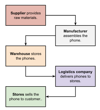
Let us take an example of mobile phone manufacturing and delivery.

Digital Twin

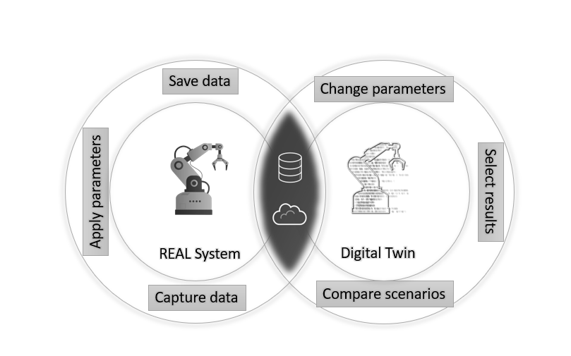
A digital twin is a virtual representation (digital model) of a real-world object, system, or process. It simulates, monitors, and analyzes the physical counterpart in real time using data collected from sensors or databases. 

Supply Chain Digital Twin

A supply chain digital twin is a real-time virtual copy of the supply chain, from raw materials to product delivery, replicating the physical processes and systems used in production, storage, and transportation. Let’s explain how the supply chain digital twins represent the complete end-to-end operations, from production to store delivery. 

Let us see some of the components and processes of each one:

• Warehouse: Location, capacity, products, etc.
• Transportation: Routes, capacity, truck id., etc.
• Stores: Location, stocks, products, etc.

Here, in the supply chain digital twins, four major analytics modules are applied: 

1. Descriptive analytics
2. Diagnostic analytics
3. Predictive analytics
4. Prescriptive analytics

Table 1: Example analytics for some cases

Implementation of Supply Chain Digital Twins Using Python

Step 1: Import Libraries

Purpose

To set up the environment with the required data analysis, simulation, and plotting tools.

Libraries Imported

• Pandas (pd): This handles tabular data in DataFrames.
• numpy (np): For numerical operations and array manipulations.
• matplotlib.pyplot (plt): For creating plots to visualize simulation results.
• Seaborn (sns): This is for enhanced visualizations (though it is not used in this notebook).
• datetime.timedelta: This is used to handle date and time operations, particularly for date-based simulations.
• This cell does not process data or produce output; it only loads dependencies.

import pandas as pd
import numpy as np
import matplotlib.pyplot as plt
import seaborn as sns
from datetime import timedelta

Step 2: Load Data and Define Products

Purpose

To load the input datasets into DataFrames and initialize the product list for the supply chain simulation.

• Data loading:
  • df_store: Loads store_daily_master.csv, parsing the date column as a datetime object. Expected to contain columns like store_name, date, inventory_{product}, and demand_{product} for each store.
  • df_warehouse: Loads warehouse_daily_master.csv, parsing the date column as a datetime object. Likely contains warehouse inventory data.
  • df_ship: Loads shipment_transportation_dataset.csv, parsing shipment_date and expected_delivery_date as datetime objects. It likely includes shipment details.
• PRODUCTS: Defines a list ['ProductA', 'ProductB', 'ProductC'] to represent the products tracked in the simulation.

The data is assumed to be pre-formatted with consistent column names (e.g., inventory_ProductA, demand_ProductA).

# --- Load Data ---
df_store = pd.read_csv("store_daily_master.csv", parse_dates=["date"])
df_warehouse = pd.read_csv("warehouse_daily_master.csv", parse_dates=["date"])
df_ship = pd.read_csv("shipment_transportation_dataset.csv", parse_dates=["shipment_date", "expected_delivery_date"])
PRODUCTS = ['ProductA', 'ProductB', 'ProductC']

Step 3: Define SupplyChainDigitalTwin Class

Purpose

To create a digital twin model for simulating daily supply chain operations and analyzing metrics like stockouts, fill rates, and reorder decisions under different demand and inventory scenarios.

• Class initialization (__init__):
  • Takes three DataFrames (store_df, warehouse_df, shipment_df) and creates deep copies to avoid modifying the original data.
  • Initializes an empty sim_results DataFrame to store simulation outputs.
• Simulation methods:
  • simulate_day(date, demand_multiplier, inventory_rule):
  • Simulates operations for a specific date.
  • Adjusts demand using demand_multiplier (e.g., 1.0 for normal, 1.5 for high demand).
  • Sets reorder_point to 60 (good policy) or 10 (bad policy, causing stockouts).
  • For each store and product, calculates:
    • Sales: min(inventory, demand)
    • Stockout: 1 if inventory < demand, else 0
    • Fill Rate: Sales/demand (1.0 if demand is 0)
    • Reorder: 1 if inventory < reorder_point, else 0
  • run_simulation(demand_multiplier, inventory_rule):
    • Iterates over unique dates in store DataFrame, calling simulate_day for each.
    • Concatenates results into self.sim_results.
• Analytics methods:
  • descriptive_analytics(): Computes stockout and fill rates and identifies stores with the most stockouts.
  • diagnostic_analytics(): Identifies days with the highest stockouts for each product.
  • predictive_analytics(): Analyzes correlations between lagged stockouts and current fill rates.
  • prescriptive_analytics(): Recommends increasing reorder points for stores with stockout rates > 10%.
• Plotting methods:
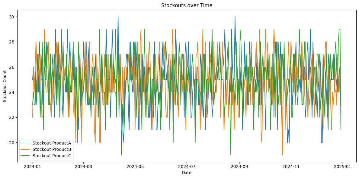
  • plot_stockouts(): Plots stockout counts over time for each product.
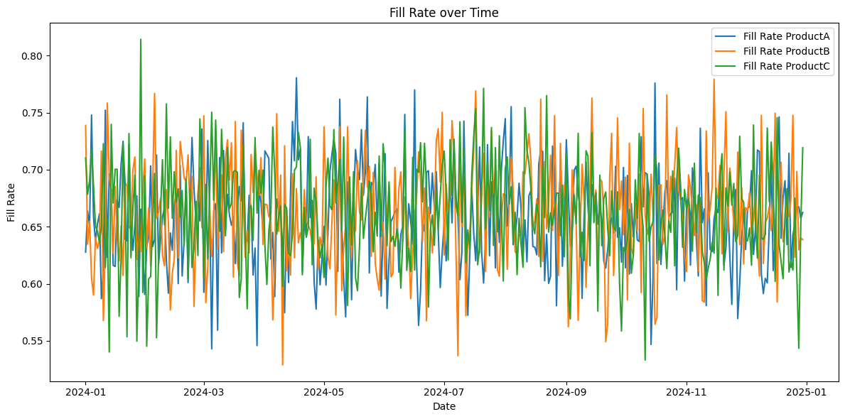
  • plot_fill_rates(): Plots average fill rates over time for each product.
  • plot_impact_of_demand_variability(): Compares total stockouts across four scenarios (normal/high demand, good/bad inventory rules).
  • The class assumes specific column names in the input DataFrames (e.g., inventory_ProductA, demand_ProductA).

# --- Digital Twin Simulation Core ---
class SupplyChainDigitalTwin:
    def __init__(self, store_df, warehouse_df, shipment_df):
        self.store = store_df.copy()
        self.warehouse = warehouse_df.copy()
        self.shipment = shipment_df.copy()
        self.sim_results = pd.DataFrame()
        
    def simulate_day(self, date, demand_multiplier=1.0, inventory_rule="good"):
        today_store = self.store[self.store['date'] == date].copy()
        today_warehouse = self.warehouse[self.warehouse['date'] == date].copy()
        
        # Apply demand scenario
        for p in PRODUCTS:
            today_store[f'demand_{p}'] = (today_store[f'demand_{p}'] * demand_multiplier).astype(int)

        # Apply inventory policy
        if inventory_rule == "bad":
            reorder_point = 10   # Too low, causes stockouts
        else:
            reorder_point = 60   # Reasonable value

        # Stockout, fill rate, and shipment simulation
        results = []
        for idx, row in today_store.iterrows():
            store_name = row['store_name']
            res = {
                "store_name": store_name,
                "date": date,
            }
            for p in PRODUCTS:
                inv = row[f'inventory_{p}']
                dem = row[f'demand_{p}']
                # Simulate sales (stockout if inv < demand)
                sales = min(inv, dem)
                stockout = int(inv < dem)
                fill_rate = sales / dem if dem > 0 else 1.0
                # Inventory policy: reorder if below point
                reorder = int(inv < reorder_point)
                res[f'sales_{p}'] = sales
                res[f'stockout_{p}'] = stockout
                res[f'fill_rate_{p}'] = fill_rate
                res[f'reorder_{p}'] = reorder
            results.append(res)
        return pd.DataFrame(results)

    def run_simulation(self, demand_multiplier=1.0, inventory_rule="good"):
        sim_frames = []
        for date in sorted(self.store['date'].unique()):
            df = self.simulate_day(date, demand_multiplier, inventory_rule)
            sim_frames.append(df)
        self.sim_results = pd.concat(sim_frames, ignore_index=True)

    # --- Analytics ---
    def descriptive_analytics(self):
        print("\n----- DESCRIPTIVE ANALYTICS -----")
        df = self.sim_results
        for p in PRODUCTS:
            print(f"{p} Stockout Rate: {df[f'stockout_{p}'].mean():.2%}")
            print(f"{p} Fill Rate: {df[f'fill_rate_{p}'].mean():.2%}")
        print("Top 5 stores with most stockouts:")
        df['total_stockouts'] = df[[f'stockout_{p}' for p in PRODUCTS]].sum(axis=1)
        print(df.groupby('store_name')['total_stockouts'].sum().sort_values(ascending=False).head())

    def diagnostic_analytics(self):
        print("\n----- DIAGNOSTIC ANALYTICS -----")
        df = self.sim_results
        # Example: Which days had most stockouts and for which products?
        by_date = df.groupby('date')[[f'stockout_{p}' for p in PRODUCTS]].sum()
        print("Days with highest stockouts:\n", by_date.sort_values(by=f'stockout_ProductA', ascending=False).head())

    def predictive_analytics(self):
        print("\n----- PREDICTIVE ANALYTICS -----")
        # Simple prediction: next day's stockout rate based on current demand/inventory
        df = self.sim_results
        for p in PRODUCTS:
            df[f'lag_stockout_{p}'] = df.groupby('store_name')[f'stockout_{p}'].shift(1)
            pred = df[[f'fill_rate_{p}', f'lag_stockout_{p}']].dropna().corr()
            print(f"Correlation between yesterday's stockout and today's fill rate for {p}:\n{pred}")

    def prescriptive_analytics(self):
        print("\n----- PRESCRIPTIVE ANALYTICS -----")
        # Recommend: Increase reorder point for stores with frequent stockouts
        df = self.sim_results
        rec_stores = df.groupby('store_name')[[f'stockout_{p}' for p in PRODUCTS]].mean()
        for p in PRODUCTS:
            prob = rec_stores[f'stockout_{p}'] > 0.1  # If stockout > 10%
            stores = rec_stores[prob].index.tolist()
            if stores:
                print(f"For {p}, recommend increasing reorder point at stores: {stores}")

    # --- Plotting ---
    def plot_stockouts(self, title="Stockouts over Time"):
        df = self.sim_results
        by_date = df.groupby('date')[[f'stockout_{p}' for p in PRODUCTS]].sum().reset_index()
        plt.figure(figsize=(12,6))
        for p in PRODUCTS:
            plt.plot(by_date['date'], by_date[f'stockout_{p}'], label=f'Stockout {p}')
        plt.xlabel("Date"); plt.ylabel("Stockout Count")
        plt.title(title)
        plt.legend(); plt.tight_layout()
        plt.show()

    def plot_fill_rates(self, title="Fill Rate over Time"):
        df = self.sim_results
        by_date = df.groupby('date')[[f'fill_rate_{p}' for p in PRODUCTS]].mean().reset_index()
        plt.figure(figsize=(12,6))
        for p in PRODUCTS:
            plt.plot(by_date['date'], by_date[f'fill_rate_{p}'], label=f'Fill Rate {p}')
        plt.xlabel("Date"); plt.ylabel("Fill Rate")
        plt.title(title)
        plt.legend(); plt.tight_layout()
        plt.show()

    def plot_impact_of_demand_variability(self):
        # Run with normal demand, then with spike, for both good and bad inventory rules
        scenarios = [
            (1.0, "good", "Base Demand, Good Rule"),
            (1.0, "bad", "Base Demand, Bad Rule"),
            (1.5, "good", "High Demand, Good Rule"),
            (1.5, "bad", "High Demand, Bad Rule")
        ]
        plt.figure(figsize=(12, 8))
        for i, (d_mult, inv_rule, label) in enumerate(scenarios):
            self.run_simulation(demand_multiplier=d_mult, inventory_rule=inv_rule)
            df = self.sim_results
            by_date = df.groupby('date')[[f'stockout_{p}' for p in PRODUCTS]].sum().sum(axis=1).reset_index(drop=True)
            plt.plot(by_date, label=label)
        plt.xlabel("Day")
        plt.ylabel("Total Stockouts (all products)")
        plt.title("Impact of Demand Variability & Bad Inventory Rule on Stockouts")
        plt.legend()
        plt.tight_layout()
        plt.show()

Step 4: Initialize SupplyChainDigitalTwin

Purpose

To instantiate the digital twin model with the store, warehouse, and shipment datasets for subsequent simulations and analyses.

• Initializes a twin object by passing df_store, df_warehouse, and df_ship to the SupplyChainDigitalTwin constructor.
• Creates copies of the input DataFrames and sets up an empty sim_results DataFrame.

# --- MAIN EXECUTION ---
twin = SupplyChainDigitalTwin(df_store, df_warehouse, df_ship)

Step 5: Run Base Simulation and Descriptive Analytics

Purpose

To simulate the supply chain under normal demand and a good inventory policy, then provide a summary of stockout rates, fill rates, and problematic stores.

• Calls twin.run_simulation() with default parameters (demand_multiplier=1.0, inventory_rule="good") to simulate operations for all dates.
• Calls twin.descriptive_analytics() to:
  • Calculate and print the mean stockout rate (stockout_{product}.mean()) for each product.
  • Calculate and print the mean fill rate (fill_rate_{product}.mean()) for each product.
  • Sum stockouts across products for each store and print the top 5 stores with the most stockouts.

# Base case: run simulation
twin.run_simulation()
twin.descriptive_analytics()

Step 6. Diagnostic Analytics

Purpose

To pinpoint specific dates and products with significant stockout issues for further investigation.

• Calls twin.diagnostic_analytics() to:
  • Group simulation results by date and sum stockouts for each product (stockout_{product}).
  • Sort by stockout_ProductA in descending order and print the top 5 days with their stockout counts for all products.

twin.diagnostic_analytics()

Step 7: Predictive Analytics

Purpose

To explore whether past stockouts can predict current fill rates, providing insights into potential patterns.

• Calls twin.predictive_analytics() to:
  • Create lagged stockout columns (lag_stockout_{product}) by shifting stockout_{product} by one day within each store.
  • Compute the correlation matrix between fill_rate_{product} and lag_stockout_{product} for each product.
  • Print the correlation matrix for each product.

twin.predictive_analytics()

Step 8: Prescriptive Analytics

Purpose

To suggest actionable improvements, specifically increasing reorder points for stores with frequent stockouts.

• Calls twin.prescriptive_analytics() to:
  • Group simulation results are calculated by store_name, and mean stockout rates for each product are calculated.
  • Identify stores where the stockout rate exceeds 10% (stockout_{product} > 0.1).
  • Print recommendations to increase reorder points for those stores.

twin.prescriptive_analytics()

Step 9: Plot Out of Sock and Fill Rates

Purpose

To visualize how fill rates and out-of-stocks (sales/demand) vary over time, helping identify trends or periods of poor performance.

• Calls twin.plot_fill_rates() and twin.plot_stockouts() to:
  • Group simulation results by date and calculate each product's mean fill_rate_{product}.
  • Create a line plot using matplotlib with:
    • X-axis: Dates
    • Y-axis: Fill Rate and out-of-stock rates (0 to 1)
    • Separate lines for ProductA, ProductB, and ProductC, labeled in the legend.
    • Figure size: 12x6 inches.
  • Add labels, title ("Fill Rate over Time"), legend, and adjust layout for clarity.

twin.plot_stockouts()
twin.plot_fill_rates()

Here, we have created sample datasets on warehouse, transportation, and store data structures for one year. These plots were generated for the supply chain digital twins on the datasets, as shown below:

Conclusion

This article discusses implementing digital twin technology in supply chain management. The outcome of this implementation shows how to boost the operation, tracking, and automation of manual jobs to avoid any unforeseen circumstances in a complete supply chain ecosystem. As a result, having a digital twin (DT) can automate all levels of information generated at any point in real time. 

This PoC can be a boon for supply chain analysts as they leverage advanced technologies such as artificial intelligence and big data analytics, and increase supply chain management (SCM) efficiency.