Feed-Forward Neural Networks With mxnetR

This is the third part of our Deep Learning series. The first in the series was Dive Deep Into Deep Learning, which focused on the basics of Deep Learning. The second was on using the H2O Deep Learning package as an autoencoder to create an anomaly detector. 

In this piece, we are going to introduce you to feed-forward neural networks. This part will focus on mxnetR, an open-source Deep Learning package that works with all Deep Learning flavors: feed-forward neural networks (FNN), convoluted neural networks (CNN), and recurrent neural networks (RNN).

Feed-Forward Neural Networks

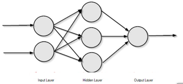
To start with a formal definition, a feed-forward neural network (AKA a multilayer perceptron, or MLP) consists of a large number of simple processing units called perceptrons organized in multiple hidden layers. To reiterate what I described in my earlier post:

• The input layer consists of neurons that accept the input values. The output from these neurons is same as the input predictors.

• The output layer is the final layer of a neural network that returns the result back to the user environment. Based on the design of a neural network, it also signals the previous layers
  on how they have performed in learning the information and accordingly improved their functions.

• Hidden layers are in between input and output layers. Typically, the number of hidden layers ranges from one to many. These are the central computation layers that have the functions that map the input to the output of a node.  

We can say a perceptron is the basic processing unit of an artificial neural network. A perceptron takes several inputs and produces an output, as shown in below figure. 

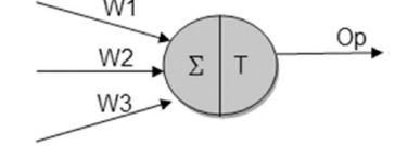
Typically, the inputs to these perceptrons are associated with a weight. A perceptron computes a weighted sum of inputs and applies a certain function to it. This function is called an activation or transfer function. The transfer function transforms the result of the summation output to a working output using mathematical functions.

Mostly, transfer functions are differential functions to enable continuous error correction and compute local gradients — such as sigmoid or tanh. This resembles real neurons that output probabilities for all output classes. However, they can typically also be a step function in which the output is set at two levels based on certain thresholds. There is also the third kind for linear units, in which the output is proportional to the total weighted output. Wikipedia has a complete list of activation functions.

The best part of a neural network is that the neurons adapt to learn from the errors and improve their results. Various methods are incorporated into a neural network to make it adaptive. The most used ones are the Delta rule and the back error propagation. The former is used in feed-forward networks and is based on the gradient descent learning, and the latter, in feedback networks such as recurrent neural networks.

I have explained a bit more about neural networks in my book Data Science Using Oracle Data Miner and Oracle R Enterprise (published by Apress).

Getting Started With MXNet Using R

As described earlier, MXNet is a deep neural net that contains feed-forward neural networks (FNN), convolution neural networks (CNN), and recurrent neural networks (RNN). CNN and RNN using MXNet are a part of the discussion for future articles.

The MXNet R package brings flexible and efficient GPU computing and state-of-art Deep Learning to R. Though we demonstrate MXNet using R, it is also supported by various other languages such as Python, Julia, C++, and Scala. So, if you're not interested in R, try this example using your favorite programming language.

MXNet installation in R is very straight-forward. You can run the below script directly in your R environment to set it up.

# Installation
 install.packages("drat", repos="https://cran.rstudio.com")
 drat:::addRepo("dmlc")
 install.packages("mxnet")

However, for Windows 7 users, there is a version issue with its one of the components DiagrammeR. You can downgrade it to v 0.8.1 using the below command. If you encounter any other issue, the MXNet website has a list of common installation problems.

install_version("DiagrammeR", version = "0.8.1", repos = "http://cran.us.r-project.org")

Creating Deep Learning Models With MXNet

We are all set to explore MXNet in R. I am using Kaggle's HR analytics data set for this demonstration. The data set is a small sample of around 14,999 rows. You can try it out with other data sets after you have learned how to use MXNet to build a feed-forward network. Our intention in this article is to help you understand and get started with MXNet.

library(mxnet)
hr_data <- read.csv("F:/git/deep_learning/mxnet/hrdata/HR.csv")
head(hr_data)
str(hr_data)
summary(hr_data)

Next, we will perform some necessary data pre-processing and partition the data into training and test sets. The training data set will be used to train a model and test data set to verify the accuracy of the newly trained model.

#Convert some variables to factors
 hr_data$sales<-as.factor(hr_data$sales)
 hr_data$salary<-as.factor(hr_data$salary)
 hr_data$Work_accident <-as.factor(hr_data$Work_accident)
 hr_data$promotion_last_5years <-as.factor(hr_data$promotion_last_5years)
 smp_size <- floor(0.70 * nrow(hr_data))

## set the seed to make your partition reproductible
 set.seed(1)
 train_ind <- sample(seq_len(nrow(hr_data)), size = smp_size)

 train <- hr_data[train_ind, ]
 test <- hr_data[-train_ind, ]

 train.preds <- data.matrix(train[,! colnames(hr_data) %in% c("left")])
 train.target <- train$left
 head(train.preds)
 head(train.target)

 test.preds <- data.matrix(test[,! colnames(hr_data) %in% c("left")])
 test.target <- test$left
 head(test.preds)
 head(test.target)

To create a feed-forward network, you can directly use mx.mlp, which is a convenient interface for creating multiple-layer perceptrons. The parameters descriptions are in comments for each used parameter.

#set seed to reproduce results
 mx.set.seed(1)

  mlpmodel <- mx.mlp(data = train.preds
   ,label = train.target
   ,hidden_node = c(3,2) #two layers — first layer with 3 nodes and second with 2 nodes
   ,out_node = 2 #number of output nodes
   ,activation="sigmoid" #activation function for hidden layers
   ,out_activation = "softmax" 
   ,num.round = 10 #number of iterations
   ,array.batch.size = 5 #batch size for updating weights
   ,learning.rate = 0.03 #same as step size
   ,eval.metric= mx.metric.accuracy
   ,eval.data = list(data = test.preds, label = test.target))

Once the training is complete, you can use the predict method to make predictions on the test data set:

#make a prediction
 preds <- predict(mlpmodel, test.x)
 dim(preds)

The function mx.mlp() is essentially a substitute to a more flexible but lengthy symbol system of defining a neural network using MXNet. The symbol is the building block a neural network in MXNet. It is a type of functional object that can take in several input variables and produce more than one output variable. Individual symbols can be stacked up on one another to produce complex symbol. This helps in formulating a complex neural network with various layers with each layer being defined as individual symbols stacked up on one another.

The equivalent of the previous network in symbolic definition will be:

#configure the network structure
 data <- mx.symbol.Variable("data")
 fc1 <- mx.symbol.FullyConnected(data, name = "fc1", num_hidden=3) #first hidden layer with activation function sigmoid
 act1 <- mx.symbol.Activation(fc1, name = "sig", act_type="sigmoid") 
 fc2 <- mx.symbol.FullyConnected(act1, name = "fc2", num_hidden=2) #second hidden layer with activation function relu
 act2 <- mx.symbol.Activation(fc2, name = "relu", act_type="relu") 
 out <- mx.symbol.SoftmaxOutput(act2, name = "soft")

#train the network
 dp_model <- mx.model.FeedForward.create(symbol = out
  ,X = train.preds
  ,y = train.target
  ,ctx = mx.cpu()
  ,num.round = 10
  ,eval.metric = mx.metric.accuracy
  ,array.batch.size = 50
  ,learning.rate = 0.005
  ,eval.data = list(data = test.preds, label = test.target))

This type of configuration gives flexibility to configure a network with different parameters for multiple hidden layers. For example, we can use the sigmoid activation function for Layer 1, the relu for Layer two, and so on.

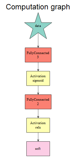
You can also visualy inspect the neural network that is created using the below code snippet:

graph.viz(mlpmodel$symbol$as.json()) 

The computation graph shows the structure of defined neural network. We can see the first hidden layer with three nodes with the sigmoid activation function, the second hidden layer with two nodes with the relu activation function, and the final output with the softmax function.

Towards the end, we can use the same predict API for creating the predictions and create a confusion matrix to establish the accuracy of the predictions on the new data set.

#make a prediction
preds <- predict(dp_model, test.preds)
preds.target <- apply(data.frame(preds[1,]), 1, function(x) {ifelse(x >0.5, 1, 0)})
table(test.target,preds.target)

You can fork and download the code from my GitHub page. We have some more articles on MXNet on creating CNN and RNN coming. In the meantime, you can explore MXNet's excellent tutorials.