Understanding Neural Networks

A comprehensive guide to the basics of neural networks, their architecture, and their types. Discover how AI mimics human senses with real-world applications.

Akash Lomas

Dec. 02, 24 · Analysis

Likes (4)

Comment

Save

2.8K Views

Artificial intelligence (AI) is designed to mimic human cognitive abilities, with many of its applications inspired by our five senses — sight, hearing, touch, taste, and smell. In AI, vision corresponds to computer vision, enabling machines to interpret images and videos. Hearing is replicated by natural language processing (NLP) and speech recognition systems, allowing AI to understand and generate human speech. Touch is simulated through haptic feedback and robotics, which help machines respond to physical interactions. Although less advanced, taste and smell are explored through AI-driven chemical analysis and sensors for food and fragrance applications.

At the core of many of these AI applications are neural networks, computational models inspired by the human brain. Neural networks consist of layers of interconnected nodes (neurons) that process data in ways similar to how the human brain works. They learn from data, identifying patterns that allow AI to make decisions, recognize images, or understand language. The deeper the network (more layers), the more sophisticated the AI’s ability to solve complex tasks. This architecture powers a broad range of AI technologies, from self-driving cars to voice assistants.

Neural networks are essential in bridging AI’s imitation of human senses and enabling more human-like intelligence. Neural networks power everything from our smartphone’s face recognition to autonomous vehicles. Whether we’re a curious beginner or an aspiring data scientist, this guide will help us understand these fascinating systems that are revolutionizing technology.

What Are Neural Networks?

Neural networks are computing systems inspired by the biological neural networks in human brains. Just as our brain consists of billions of interconnected neurons that help us learn and make decisions, artificial neural networks are digital systems that learn from experience.

Basic Components

A neural network is a network of neurons. Let's understand its basic components.

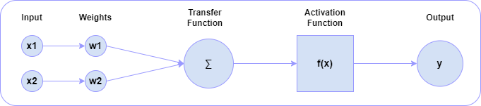
1. Neurons (Nodes)

Process input signals.
Apply weights and biases.
Use activation functions to produce output.

2. Connections (Weights)

Represent the strength of connections between neurons.
Adjust during learning.
Determine network behavior.

3. Layers

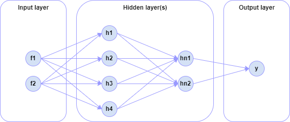
Input Layer

The data that we feed to the model is loaded into the input layer from external sources like a CSV file or a web service. It is the only visible layer in the complete neural network architecture that passes the complete information from the outside world without any computation.

Hidden Layers

The hidden layers are what make deep learning what it is today. They are intermediate layers that do all the computations and extract the features from the data.

There can be multiple interconnected hidden layers that account for searching different hidden features in the data. For example, in image processing, the first hidden layers are responsible for higher-level features like edges, shapes, or boundaries. On the other hand, the later hidden layers perform more complicated tasks like identifying complete objects (a car, a building, a person).

Output Layer

The output layer takes input from preceding hidden layers and comes to a final prediction based on the model’s learning. It is the most important layer where we get the final result.

In the case of classification/regression models, the output layer generally has a single node. However, it is completely problem-specific and dependent on the way the model was built.

Types of Neural Networks

1. Feed-Forward Neural Networks (FNN)

Simplest architecture.
Information flows in one direction.
Good for structured data and classification.
Example use: Credit risk assessment.

2. Convolutional Neural Networks (CNN)

Specialized for processing grid-like data.
Excellent for image and video processing.
Uses convolution operations.
Example use: Face recognition, medical imaging.

3. Recurrent Neural Networks (RNN)

Processes sequential data.
Has internal memory.
Good for time-series data.
Example use: Stock price prediction.

4. Long Short-Term Memory Networks (LSTM)

Advanced RNN variant.
Better at handling long-term dependencies.
Contains special memory cells.
Example use: Language translation, speech recognition.

How Are Neural Networks Created?

Architecture Design

1. Simple Feedforward Neural Network (FNN)

This model is designed for simple tasks like digit classification:

    Python
   
 

   import tensorflow as tf

def create_basic_nn():
    return tf.keras.Sequential([
        tf.keras.layers.Dense(128, activation='relu', input_shape=(784,)),
        tf.keras.layers.Dropout(0.2),
        tf.keras.layers.Dense(64, activation='relu'),
        tf.keras.layers.Dense(10, activation='softmax')
    ])
  

2. Convolutional Neural Network (CNN) for Image Processing

This architecture is tailored for tasks like image recognition and processing:

    Python
   
 

   def create_cnn():
    return tf.keras.Sequential([
        tf.keras.layers.Conv2D(32, (3, 3), activation='relu', input_shape=(28, 28, 1)),
        tf.keras.layers.MaxPooling2D((2, 2)),
        tf.keras.layers.Conv2D(64, (3, 3), activation='relu'),
        tf.keras.layers.MaxPooling2D((2, 2)),
        tf.keras.layers.Flatten(),
        tf.keras.layers.Dense(64, activation='relu'),
        tf.keras.layers.Dense(10, activation='softmax')
    ])
  

How Do Neural Networks Learn?

The Learning Process

1. Forward Pass

    Python
   
   def forward_pass(model, inputs):
  # Make predictions
  predictions = model(inputs)
  return predictions

2. Error Calculation

    Python
   
 

   def calculate_loss(predictions, actual):
  # Using categorical crossentropy
  loss_object = tf.keras.losses.CategoricalCrossentropy()
  loss = loss_object(actual, predictions)
  return loss
  

3. Backpropagation and Optimization

    Python
   
 

   # Complete training example
def train_model(model, x_train, y_train):

  # Prepare data
  x_train = x_train.reshape(-1, 784).astype('float32') / 255.0
  
  # Compile model
  model.compile(
    optimizer=tf.keras.optimizers.Adam(learning_rate=0.001),
    loss='sparse_categorical_crossentropy',
    metrics=['accuracy']
    )
  
  # Train
  history = model.fit(
    x_train, y_train,
    epochs=10,
    validation_split=0.2,
    batch_size=32,
    callbacks=[
    tf.keras.callbacks.EarlyStopping(patience=3),
    tf.keras.callbacks.ReduceLROnPlateau()
    ])
  return history
  

Optimization Techniques

1. Batch Processing

Mini-batch gradient descent.
Batch normalization.
Gradient clipping.

2. Regularization

Dropout.
L1/L2 regularization.
Data augmentation.

Evaluating Neural Networks

Performance Metrics

    Python
   
   def evaluate_model(model, x_test, y_test):
  # Basic metrics
  test_loss, test_accuracy = model.evaluate(x_test, y_test)
  
  # Detailed metrics
  predictions = model.predict(x_test)
  
  from sklearn.metrics import classification_report, confusion_matrix
  
  print(classification_report(y_test.argmax(axis=1), predictions.argmax(axis=1)))
  print("\nConfusion Matrix:")
  print(confusion_matrix(y_test.argmax(axis=1), predictions.argmax(axis=1)))

Common Challenges and Solutions

1. Overfitting

Symptoms: High training accuracy, low validation accuracy
Solutions:

    Python
   
   # Add regularization
tf.keras.layers.Dense(64, activation='relu',
  kernel_regularizer=tf.keras.regularizers.l2(0.01))

# Add dropout
tf.keras.layers.Dropout(0.5)

2. Underfitting

Symptoms: Low training and validation accuracy
Solutions:
- Increase model capacity
- Add more layers
- Increase training time

Neural Networks vs. Transformers

Key Differences

1. Architecture

Traditional RNN:

    Python
   
 

   def create_rnn():
  return tf.keras.Sequential([
    tf.keras.layers.LSTM(64, return_sequences=True),
    tf.keras.layers.LSTM(32),
    tf.keras.layers.Dense(10)
  ])
  

Simple Transformer:

    Python
   
 

   def create_transformer():
  return tf.keras.Sequential([
    tf.keras.layers.MultiHeadAttention(num_heads=8, key_dim=64),
    tf.keras.layers.LayerNormalization(),
    tf.keras.layers.Dense(64, activation='relu'),
    tf.keras.layers.Dense(10)
  ])
  

2. Processing Capabilities

Neural Networks: Sequential processing.
Transformers: Parallel processing with attention mechanism.

3. Use Cases

Neural Networks: Traditional ML tasks, computer vision.
Transformers: NLP, large-scale language models.

Practical Implementation Tips

1. Model Selection

    Python
   
 

   def choose_model(task_type, input_shape):
  if task_type == 'image':
    return create_cnn()
  elif task_type == 'sequence':
    return create_rnn()
  else:
    return create_basic_nn()
  

2. Hyperparameter Tuning

    Python
   
 

   from keras_tuner import RandomSearch

def tune_hyperparameters(model_builder, x_train, y_train):
  tuner = RandomSearch(
    model_builder,
    objective='val_accuracy',
    max_trials=5
    )
  tuner.search(x_train, y_train,
  epochs=5,
  validation_split=0.2)
  return tuner.get_best_hyperparameters()[0]
  

Real-World Case Studies

1. Medical Image Analysis

Example: COVID-19 X-ray Classification:

    Python
   
 

   def create_medical_cnn():
  model = tf.keras.Sequential([
    tf.keras.layers.Conv2D(32, (3, 3), activation='relu', input_shape=(224, 224, 3)),
    tf.keras.layers.BatchNormalization(),
    tf.keras.layers.MaxPooling2D((2, 2)),
    tf.keras.layers.Conv2D(64, (3, 3), activation='relu'),
    tf.keras.layers.BatchNormalization(),
    tf.keras.layers.MaxPooling2D((2, 2)),
    tf.keras.layers.Conv2D(128, (3, 3), activation='relu'),
    tf.keras.layers.BatchNormalization(),
    tf.keras.layers.GlobalAveragePooling2D(),
    tf.keras.layers.Dense(2, activation='softmax')
  ])
  return model
  

Custom data generator with augmentation:

    Python
   
 

   def create_medical_data_generator():
  return tf.keras.preprocessing.image.ImageDataGenerator(
    rotation_range=20,
    width_shift_range=0.2,
    height_shift_range=0.2,
    horizontal_flip=True,
    validation_split=0.2,
    preprocessing_function=tf.keras.applications.resnet50.preprocess_input
  )
  

2. Financial Time Series Prediction

Example: Stock Price Prediction:

    Python
   
 

   def create_financial_lstm():
  model = tf.keras.Sequential([
    tf.keras.layers.LSTM(50, return_sequences=True, input_shape=(60, 5)),
    tf.keras.layers.Dropout(0.2),
    tf.keras.layers.LSTM(50, return_sequences=False),
    tf.keras.layers.Dropout(0.2),
    tf.keras.layers.Dense(1)])
  return
  

Feature engineering for financial data:

    Python
   
 

   def prepare_financial_data(df, look_back=60):
  features = ['Open', 'High', 'Low', 'Close', 'Volume']
  scaler = MinMaxScaler()
  scaled_data = scaler.fit_transform(df[features])
  X, y = [], []

  for i in range(look_back, len(scaled_data)):
    X.append(scaled_data[i-look_back:i])
    y.append(scaled_data[i, 3]) # Predicting Close price
    return np.array(X), np.array(y), scaler
  

Model Deployment Guide

1. Model Optimization

Quantization:

    Python
   
 

   def quantize_model(model):
  converter = tf.lite.TFLiteConverter.from_keras_model(model)
  converter.optimizations = [tf.lite.Optimize.DEFAULT]
  converter.target_spec.supported_types = [tf.float16]
  tflite_model = converter.convert()
  return tflite_model
  

Pruning:

    Python
   
 

   def create_pruned_model(model, training_data):
  pruning_params = {
    'pruning_schedule': tfmot.sparsity.keras.PolynomialDecay(
    initial_sparsity=0.30,
    final_sparsity=0.80,
    begin_step=0,
    end_step=end_step)
  }
  model_pruned = tfmot.sparsity.keras.prune_low_magnitude(
  model, pruning_params)
  return model_pruned
  

2. Production Deployment

Flask API for model serving:

    Python
   
 

   from flask import Flask, request, jsonify

app = Flask(__name__)
model = None

def load_model():
  global model
  model = tf.keras.models.load_model('path/to/model')
  @app.route('/predict', methods=['POST'])

def predict():
  data = request.json['data']
  processed_data = preprocess_input(data)
  prediction = model.predict(processed_data)
  return jsonify({'prediction': prediction.tolist()})
  

Dockerfile:

    Python
   
   FROM python:3.8-slim

WORKDIR /app

COPY requirements.txt .
RUN pip install -r requirements.txt

COPY . .
CMD ["python", "app.py"]

Latest Architectural Innovations

1. Vision Transformers (ViT)

    Python
   
 

   def create_vit_model(input_shape, num_classes):
  inputs = tf.keras.Input(shape=input_shape)
  
  # Patch embedding
  patches = tf.keras.layers.Conv2D(filters=768, kernel_size=16, strides=16)(inputs)
  flat_patches = tf.keras.layers.Reshape((-1, 768))(patches)
  
  # Position embedding
  positions = tf.range(start=0, limit=flat_patches.shape[1], delta=1)
  pos_embedding = tf.keras.layers.Embedding(input_dim=flat_patches.shape[1], output_dim=768)(positions)
  x = flat_patches + pos_embedding
  
  # Transformer blocks
  for _ in range(12):
    x = transformer_block(x)
    x = tf.keras.layers.GlobalAveragePooling1D()(x)
    outputs = tf.keras.layers.Dense(num_classes, activation='softmax')(x)
    return tf.keras.Model(inputs=inputs, outputs=outputs)
  

2. MLP-Mixer Architecture

    Python
   
 

   def mlp_block(x, hidden_units, dropout_rate):
  x = tf.keras.layers.Dense(hidden_units, activation='gelu')(x)
  x = tf.keras.layers.Dense(x.shape[-1])(x)
  x = tf.keras.layers.Dropout(dropout_rate)(x)
  return x

def mixer_block(x, tokens_mlp_dim, channels_mlp_dim, dropout_rate):
  # Token-mixing
  y = tf.keras.layers.LayerNormalization()(x)
  y = tf.transpose(y, perm=[0, 2, 1])
  y = mlp_block(y, tokens_mlp_dim, dropout_rate)
  y = tf.transpose(y, perm=[0, 2, 1])
  x = x + y
  
  # Channel-mixing
  y = tf.keras.layers.LayerNormalization()(x)
  y = mlp_block(y, channels_mlp_dim, dropout_rate)
  return x + y
  

Performance Optimization Tips

1. Memory Management

Custom data generator for large datasets:

    Python
   
 

   class DataGenerator(tf.keras.utils.Sequence):
def __init__(self, x_set, y_set, batch_size):
  self.x, self.y = x_set, y_set
  self.batch_size = batch_size

def __len__(self):
  return int(np.ceil(len(self.x) / self.batch_size))

def __getitem__(self, idx):
  batch_x = self.x[idx * self.batch_size:(idx + 1) * self.batch_size]
  batch_y = self.y[idx * self.batch_size:(idx + 1) * self.batch_size]
  return np.array(batch_x), np.array(batch_y)
  

2. Training Optimization

Mixed precision training:

    Python
   
   def enable_mixed_precision():
  policy = tf.keras.mixed_precision.Policy('mixed_float16')
  tf.keras.mixed_precision.set_global_policy(policy)

Custom training loop with gradient accumulation:

    Python
   
 

   def train_with_gradient_accumulation(model, dataset, accumulation_steps=4):
  optimizer = tf.keras.optimizers.Adam()
  gradients = [tf.zeros_like(v) for v in model.trainable_variables]
  for step, (x_batch, y_batch) in enumerate(dataset):
    with tf.GradientTape() as tape:
      predictions = model(x_batch, training=True)
      loss = compute_loss(y_batch, predictions)
      loss = loss / accumulation_steps
      grads = tape.gradient(loss, model.trainable_variables)
      gradients = [(acc_grad + grad) for acc_grad, grad in zip(gradients, grads)]
      
      if (step + 1) % accumulation_steps == 0:
        optimizer.apply_gradients(zip(gradients, model.trainable_variables))
        gradients = [tf.zeros_like(v) for v in model.trainable_variables]
  

Additional Resources

1. Online Learning Platforms

Coursera: Deep Learning Specialization
Fast.ai: Practical Deep Learning
TensorFlow Official Tutorials

2. Books

“Deep Learning” by Ian Goodfellow
“Neural Networks and Deep Learning” by Michael Nielsen

3. Practice Platforms

Kaggle: Real-world datasets and competitions
Google Colab: Free GPU access
TensorFlow Playground: Interactive visualization

Conclusion

Neural networks are powerful tools that continue to evolve. This guide provides a foundation, but the field is rapidly advancing. Keep experimenting, stay curious, and remember that practical experience is the best teacher.

Here are some tips for success:

Start with simple architectures.
Understand your data thoroughly.
Monitor training metrics carefully.
Use version control for your models.
Keep up with the latest research.

Remember: The best way to learn is by implementing and experimenting with different architectures and datasets.

neural network Neural Networks (journal) Network

Opinions expressed by DZone contributors are their own.

Related

Trending