Kullback–Leibler Divergence: Theory, Applications, and Implications
Kullback–Leibler divergence (KL divergence) is a statistical measure that quantifies how one probability distribution differs from a second reference distribution.
Join the DZone community and get the full member experience.
Join For FreeKullback–Leibler divergence (KL divergence), also known as relative entropy, is a fundamental concept in statistics and information theory. It measures how one probability distribution diverges from a second, reference probability distribution. This article delves into the mathematical foundations of KL divergence, its interpretation, properties, applications across various fields, and practical considerations for its implementation.
1. Introduction
Introduced by Solomon Kullback and Richard Leibler in 1951, KL divergence quantifies the information lost when one distribution is used to approximate another. It is widely utilized in various fields such as machine learning, statistics, fluid mechanics, neuroscience, and bioinformatics. Understanding KL divergence is essential for model comparison and inference in these domains.
2. Mathematical Foundations
2.1 Discrete Variables
For discrete random variables PP and QQ with supports XX and probability mass functions p(x)p(x) and q(x)q(x), the KL divergence from QQ to PP is defined as:
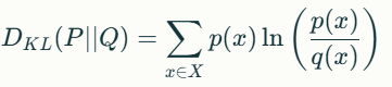
This formula captures the expected number of extra bits required to encode samples from PP using a code optimized for QQ. A zero KL divergence indicates that the two distributions are identical.
2.2 Continuous Variables
For continuous random variables, the KL divergence is expressed as:
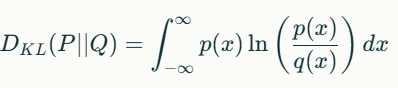
In this case, p(x)p(x) and q(x)q(x) are the probability density functions of the respective distributions.
3. Interpretation of KL Divergence
KL divergence provides insight into how well one distribution approximates another. A lower value indicates a better approximation, while a higher value signifies greater dissimilarity. The first term in the continuous case represents the entropy of the true model (the total amount of uncertainty), while the second term quantifies the cross-entropy (the uncertainty captured by the model). The difference between these two terms reflects the remaining uncertainty after using the model for approximation.
4. Properties of KL Divergence
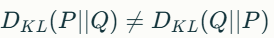
- Non-Symmetry: KL divergence is not symmetric; that is,
![]() This property can lead to different interpretations depending on which distribution is treated as the reference.
This property can lead to different interpretations depending on which distribution is treated as the reference. - Non-Negativity: The value of KL divergence is always non-negative
![]() achieving zero only when both distributions are identical.
achieving zero only when both distributions are identical. - Convexity: KL divergence is a convex function with respect to its distributions, meaning that mixing two distributions will yield a KL divergence that is less than or equal to the weighted sum of their individual divergences.
 This property can lead to different interpretations depending on which distribution is treated as the reference.
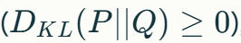 achieving zero only when both distributions are identical.
5. Applications of KL Divergence
5.1 Statistical Model Comparison
KL divergence serves as a robust metric for comparing statistical models. Researchers can select models that minimize information loss by evaluating how well a model approximates true data distributions.
When comparing two models, say Model 1 and Model 2, researchers compute the KL divergence for each model relative to the true distribution. A lower KL divergence score indicates that the model's predictions are closer to the actual data distribution, thereby minimizing information loss. For instance, if Model 1 has a KL divergence of 0.3 and Model 2 has a KL divergence of 0.4, it can be concluded that Model 1 is more effective in capturing the true data distribution than Model 2.
5.2 Variational Bayesian Inference
In Bayesian inference, KL divergence plays a crucial role in variational methods where it helps approximate complex posterior distributions by simpler ones.
KL divergence is used to measure how well the approximating distribution (often denoted as qq) matches the true posterior distribution (denoted as pp). The variational inference process involves minimizing the KL divergence between these two distributions mentioned in the section 4.
By minimizing this divergence, researchers can derive an optimal approximation of the posterior distribution that is computationally feasible to work with. This approach is particularly useful in scenarios where direct computation of the posterior is intractable due to high dimensionality or complex models. Variational Bayesian inference thus enables practitioners to perform Bayesian analysis more efficiently while maintaining a level of accuracy that is often sufficient for practical applications.
5.3 Machine Learning
In machine learning applications, KL divergence is often used in algorithms such as Generative Adversarial Networks (GANs), where it measures how well generated data matches real data distributions.
KL divergence serves as a measure of how well the generated data matches the real data distribution. The generator seeks to minimize this divergence during training, effectively learning to produce samples that are increasingly similar to those drawn from the true data distribution.
Additionally, KL divergence is closely related to other loss functions used in machine learning, such as cross-entropy loss. Both metrics quantify differences between distributions and are often interchangeable depending on the context. This makes KL divergence a valuable tool not only for evaluating model performance but also for guiding optimization processes in various machine learning algorithms.
6. Practical Considerations
When calculating KL divergence, certain challenges arise:
- Handling Zero Probabilities: If one distribution assigns zero probability to an event that has non-zero probability in another distribution, this leads to undefined or infinite KL divergence values.
To address this issue, smoothing techniques can adjust probabilities slightly above zero.
Example: Computing KL Divergence with Smoothing
Consider two sample distributions:
- P=(a:3/5,b:2/5)P=(a:3/5,b:2/5)
- Q=(a:5/9,b:3/9,d:1/9)Q=(a:5/9,b:3/9,d:1/9)
To compute DKL(P∣∣Q)DKL(P∣∣Q), we introduce a small constant ϵ=10−3ϵ=10−3:
- Create smoothed versions:
- Adjust probabilities in both distributions so that all events have non-zero probabilities.
- For instance:
- Smoothed P′=(a:3/5−ϵ/2,b:2/5−ϵ/2,d:ϵ)P′=(a:3/5−ϵ/2,b:2/5−ϵ/2,d:ϵ)
- Smoothed Q′=(a:5/9−ϵ/2,b:3/9−ϵ/2,d:1/9−ϵ/2)Q′=(a:5/9−ϵ/2,b:3/9−ϵ/2,d:1/9−ϵ/2)
- Compute smoothed KL Divergence:
Pythonimport numpy as np # Define smoothed distributions P_prime = np.array([3/5 - 0.001/2, 2/5 - 0.001/2, 0.001]) # Adding epsilon for missing event d Q_prime = np.array([5/9 - 0.001/2, 3/9 - 0.001/2, 0.001]) # Smoothing for events # Calculate KL Divergence def kl_divergence(p, q): return np.sum(p * np.log(p / q)) kl_value = kl_divergence(P_prime + np.finfo(float).eps, Q_prime + np.finfo(float).eps) print(f"Smoothed KL Divergence: {kl_value}")
7. Use Case Scenario: Monitoring Data Drift in Machine Learning Models
In the rapidly evolving landscape of data science and machine learning, maintaining the accuracy and reliability of models is paramount. One common challenge faced by data scientists is data drift, which occurs when the statistical properties of the input data change over time. This can lead to model degradation, where the model's predictions become less accurate as they are based on outdated data distributions. A practical solution to this problem is to utilize "Kullback-Leibler (KL) divergence" as a metric for monitoring data drift.
Scenario Description
Imagine a company that has deployed a machine learning model to predict customer churn based on various features such as customer demographics, transaction history, and engagement metrics. Initially, the model performs well; however, over time changes in customer behavior perhaps due to market trends or external factors result in shifts in the underlying data distribution. If not monitored properly, these changes can lead to significant drops in prediction accuracy.
Solution Using KL Divergence
To effectively monitor for data drift, the company can implement a system that calculates KL divergence between the current input feature distributions and a baseline distribution established during the model training phase. The steps involved in this solution are as follows:
- Establish Baseline Distributions: During the training phase, collect and analyze the input feature distributions to create a baseline model. This serves as a reference point for future comparisons.
- Continuous Monitoring: Implement a monitoring system that regularly collects new input data and computes the KL divergence between the current feature distributions and the baseline distributions using Python libraries such as NumPy or SciPy.
- Set Thresholds: Define thresholds for acceptable levels of KL divergence. If the KL divergence exceeds these thresholds, it indicates significant drift in the data distribution.
- Trigger Actions: If drift is detected (i.e., KL divergence exceeds the threshold), trigger automated actions such as:
- Alerting data scientists to investigate potential causes of drift.
- Initiating retraining of the model with updated data to ensure it remains accurate and relevant.
- Conducting further statistical analysis to understand which features have changed significantly.
Example Implementation
Here’s a simple example of how KL divergence can be computed using Python:
import numpy as np

from scipy.special import rel_entr

# Example baseline distribution (P) and current distribution (Q)

baseline_distribution = np.array([0.4, 0.6])  # Example: 40% A, 60% B

current_distribution = np.array([0.5, 0.5])   # Example: 50% A, 50% B

# Calculate KL Divergence

def kl_divergence(p, q):

    return np.sum(rel_entr(p, q))

# Compute KL divergence from baseline to current

kl_value = kl_divergence(baseline_distribution + 1e-10, current_distribution + 1e-10)

print(f"KL Divergence: {kl_value}")
In this code snippet:
- We define two distributions representing baseline and current states.
- The
kl_divergencefunction calculates KL divergence usingrel_entr, which computes relative entropy. - A small constant (
1e-10) is added to avoid division by zero errors when any probabilities are zero.
8. Insights into Kullback–Leibler Divergence
Understanding Kullback–Leibler divergence involves recognizing its implications in statistical modeling and machine learning contexts. A high KL divergence value indicates that there is a significant difference between the two probability distributions being compared; this means that using one distribution to approximate another will result in considerable information loss.
It’s important to note that KL divergence cannot be negative; it is always non-negative due to its mathematical formulation and properties derived from information theory.Furthermore, KL divergence relates closely to entropy itself; it consists of two components—entropy and cross-entropy—where entropy measures the uncertainty inherent in a true distribution while cross-entropy measures how well an approximating model captures that uncertainty. KL divergence proves particularly useful when comparing probabilistic models or assessing model performance in machine learning contexts like classification and generative modeling.
9. Conclusion
Kullback–Leibler divergence offers a powerful framework for understanding and quantifying differences between probability distributions. Its applications span numerous fields including machine learning and statistics where it aids in model selection and validation. By grasping its mathematical foundations and practical implications, researchers and practitioners can leverage this measure to enhance their analytical capabilities. As we continue to explore complex data-driven environments, understanding tools like KL divergence will remain crucial for effective modeling and inference.
References
- Kullback S., & Leibler R.A. (1951). "On Information and Sufficiency". Annals of Mathematical Statistics.
- Cover T.M., & Thomas J.A. (2006). "Elements of Information Theory". Wiley-Interscience.
- StatLect (2021). "Kullback-Leibler Divergence". Retrieved from StatLect website.
- Encord (2024). "KL Divergence in Machine Learning". Retrieved from Encord blog.
Published at DZone with permission of Shailendra Prajapati. See the original article here.
Opinions expressed by DZone contributors are their own.
Comments